Hamiltonian Mechanics: Problem Solving

1. The "Why" and "How" of Hamiltonian Mechanics

Before we dive into problem-solving, it's worth taking a moment to appreciate the conceptual shift that Hamiltonian mechanics represents. It's more than just a new set of equations; it's a new way of thinking about dynamics.

2. The Hamiltonian Recipe: A Step-by-Step Guide

As summarized in the video, solving a problem using the Hamiltonian formalism follows a clear, systematic procedure. This process ensures we correctly move from the configuration space of the Lagrangian ($q,\dot{q}$) to the phase space of the Hamiltonian ($q,p$).

For a system with $N$ generalized coordinates, the steps are:

1. Write the Lagrangian: Calculate the kinetic energy $T$ and potential energy $V$, and form the Lagrangian $L(q_i,{\dot{q}}_i,t)=T-V$.
2. Find the Canonical Momenta: For each coordinate $q_i$, calculate its conjugate momentum $p_i$ using the definition:
   $p_i=\frac{\partial L}{\partial {\dot{q}}_i}$
3. Invert for Velocities: Algebraically solve the $N$ equations from Step 2 to express each generalized velocity ${\dot{q}}_i$ as a function of the coordinates and momenta, ${\dot{q}}_i(q_j,p_j,t)$. This is a critical step.
4. Construct the Hamiltonian: Write the formal definition of the Hamiltonian:
   $H={\sum }_{i=1}^N{p}_i{\dot{q}}_i-L$
   Then, substitute the expressions for ${\dot{q}}_i$ from Step 3 into this equation to get the final Hamiltonian $H(q_i,p_i,t)$. No ${\dot{q}}_i$ terms should remain.
5. Write Hamilton's Equations: For each of the $N$ degrees of freedom, write down the two first-order canonical equations:
   ${\dot{q}}_i=\frac{\partial H}{\partial p_i}\text{and}{\dot{p}}_i=-\frac{\partial H}{\partial q_i}$
   This will give you a system of $2N$ first-order ordinary differential equations.
6. Solve the Equations: Solve this system of ODEs to find the motion of the system, $q_i(t)$ and $p_i(t)$. Often, this involves combining a pair of equations to eliminate $p_i$ and recover a single second-order equation for $q_i$, which is typically equivalent to the Euler-Lagrange equation.

This procedure is summarized well in the following resource, which you can use as a reference.

3. Worked Examples

Let's apply this recipe to a few physical systems.

Example 1: The Simple Pendulum

Consider a simple pendulum of mass $m$ and length $l$. The generalized coordinate is the angle $\theta$.

1. Lagrangian: The kinetic energy is $T=\frac{1}{2}m{l}^2{\dot{\theta }}^2$ and the potential energy is $V=-mgl\cos \theta$ (taking $V=0$ at the bottom).
   $L=T-V=\frac{1}{2}m{l}^2{\dot{\theta }}^2+mgl\cos \theta$

2. Canonical Momentum:
   $p_{\theta }=\frac{\partial L}{\partial \dot{\theta }}=m{l}^2\dot{\theta }$

3. Invert for Velocity:
   $\dot{\theta }=\frac{p_{\theta }}{m{l}^2}$

4. Construct Hamiltonian:
   $H=p_{\theta }\dot{\theta }-L=p_{\theta }\left(\frac{p_{\theta }}{m{l}^2}\right)-\left(\frac{1}{2}m{l}^2{\left(\frac{p_{\theta }}{m{l}^2}\right)}^2+mgl\cos \theta \right)$
   $H=\frac{p_{\theta }^2}{m{l}^2}-\left(\frac{p_{\theta }^2}{2m{l}^2}+mgl\cos \theta \right)=\frac{p_{\theta }^2}{2m{l}^2}-mgl\cos \theta$
   Notice that $T=\frac{p_{\theta }^2}{2m{l}^2}$ and the potential energy in the Hamiltonian is $-V$. In this case, $H=T+V$, the total energy.

5. Hamilton's Equations:
   $\dot{\theta }=\frac{\partial H}{\partial p_{\theta }}=\frac{p_{\theta }}{m{l}^2}$
   ${\dot{p}}_{\theta }=-\frac{\partial H}{\partial \theta }=-\frac{\partial }{\partial \theta }(-mgl\cos \theta )=-mgl\sin \theta$

6. Solve: The first equation simply confirms our expression for $\dot{\theta }$. We can differentiate it with respect to time to get $\ddot{\theta }={\dot{p}}_{\theta }/(m{l}^2)$. Substituting the second equation into this gives:
   $\ddot{\theta }=\frac{-mgl\sin \theta }{m{l}^2}⟹\ddot{\theta }+\frac{g}{l}\sin \theta =0$
   This is the familiar equation of motion for a pendulum.

The video you watched earlier contains a walkthrough of this exact problem. You can review it if any step was unclear.

Example 2: Bead on a Parabolic Wire

Let's tackle a more complex case where the canonical momentum isn't simply $m\times (\text{velocity})$. Consider a bead of mass $m$ sliding on a frictionless parabolic wire in a vertical plane, given by $y=\frac{1}{2}a{x}^2$.

1. Lagrangian:
   The velocity squared is $v^2={\dot{x}}^2+{\dot{y}}^2$. Since $y=\frac{1}{2}a{x}^2$, we have $\dot{y}=ax\dot{x}$.
   $v^2={\dot{x}}^2+(ax\dot{x}{)}^2=(1+a^2{x}^2){\dot{x}}^2$
   The Lagrangian is $L=T-V=\frac{1}{2}m(1+a^2{x}^2){\dot{x}}^2-\frac{1}{2}mga{x}^2$.

2. Canonical Momentum:
   $p_x=\frac{\partial L}{\partial \dot{x}}=m(1+a^2{x}^2)\dot{x}$
   Notice here that $p_x$ depends on both $\dot{x}$ and $x$.

The rest of the derivation involves some algebra.

Advanced Example: The Double Pendulum

To satisfy your interest in high-level problems, consider the double pendulum. Its Lagrangian (for two equal masses $m$ and lengths $l$) is already quite complex:
$L=m{l}^2{\dot{\theta }}_1^2+\frac{1}{2}m{l}^2{\dot{\theta }}_2^2+m{l}^2\cos ({\theta }_1-{\theta }_2){\dot{\theta }}_1{\dot{\theta }}_2-mgl(2\cos {\theta }_1+\cos {\theta }_2)$
Following the Hamiltonian recipe from here involves significant algebraic manipulation. The resulting Hamiltonian is:
$H=\frac{p_1^2+2p_2^2-2p_1{p}_2\cos ({\theta }_1-{\theta }_2)}{2m{l}^2{\sin }^2({\theta }_1-{\theta }_2)}-mgl(2\cos {\theta }_1+\cos {\theta }_2)$
From this $H$, one would then derive the four Hamilton's equations for ${\dot{\theta }}_1,{\dot{p}}_1,{\dot{\theta }}_2,{\dot{p}}_2$. While we won't perform the derivation here, it's a perfect example of the formalism's power to handle even very complex systems systematically. If you wish to see the full, rigorous derivation, the resource below provides it.

4. The Geometric Picture: Motion as a Flow in Phase Space

What is the ultimate payoff for this more abstract formalism? One major benefit is a new, powerful geometric interpretation of dynamics. Hamilton's equations treat coordinates ($q$) and momenta ($p$) on an equal footing. The $2N$-dimensional space spanned by all the $q_i$ and $p_i$ is called phase space.

The state of a system at any instant is represented by a single point in phase space. As time evolves, this point traces out a trajectory. Hamilton's equations, $\dot{q}=\partial H/\partial p$ and $\dot{p}=-\partial H/\partial q$, define a unique velocity vector $(\dot{q},\dot{p})$ at every point in phase space. This vector field defines a "flow," and the system's evolution is simply following this flow.

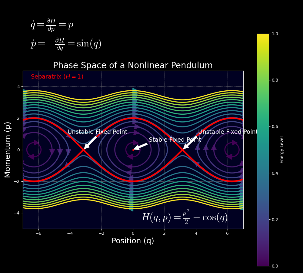
This geometric view is incredibly powerful. The structure of the phase space portrait tells you everything about the possible motions of the system without solving the equations for every initial condition.

Conclusion

In this lesson, we established a robust methodology for analyzing mechanical systems within the Hamiltonian framework. We saw how this "recipe" can be applied to simple and complex problems alike, always yielding a set of first-order differential equations that govern the system's evolution in phase space.

Key Takeaways:

• Solving problems with Hamiltonian mechanics follows a six-step recipe: L → p → $\dot{q}(p)$ → H → Hamilton's Equations → Solve.
• The crucial step is to express the Hamiltonian $H$ strictly as a function of coordinates $q$, momenta $p$, and time $t$, eliminating all generalized velocities $\dot{q}$.
• The result is a set of $2N$ first-order ODEs, in contrast to the $N$ second-order ODEs of the Lagrangian method.
• Conceptually, Hamiltonian dynamics is best viewed as a flow on phase space, where the Hamiltonian function itself generates the evolution of the system's state.

Preview of the Next Lesson:
We've just had a glimpse of the power of the phase space picture. In our next lesson, we will delve deeper into this concept. We will learn how to construct and interpret phase space diagrams for simple Hamiltonian systems, allowing us to understand the qualitative nature of a system's motion—identifying oscillations, rotations, and points of equilibrium—purely by analyzing the geometry of its phase space.