Phase Space Diagrams for Hamiltonian Systems

1. From Hamiltonian to Phase Portrait

Let's start by formalizing the connection between the Hamiltonian and the phase portrait. For a system with one degree of freedom, the phase space is a 2D plane with coordinates $(q,p)$. A phase portrait is a drawing of the trajectories (or "flow lines") that a system can follow in this space.

For a conservative system, the Hamiltonian $H(q,p)$ does not explicitly depend on time, which means the total energy is conserved. We proved this in the last lesson: if $\partial H/\partial t=0$, then $dH/dt=0$. This has a profound geometric consequence:

A system's trajectory in phase space must always stay on a curve of constant energy.

Therefore, the phase portrait is simply the set of contour lines (or level sets) of the function $H(q,p)$. To draw the portrait, we just need to plot the curves $H(q,p)=E$ for various values of energy $E$.

The direction of flow along these contours is given by Hamilton's equations, which define a "velocity" vector, or flow vector, at every point in phase space:
$\vec{v}=(\dot{q},\dot{p})=\left(\frac{\partial H}{\partial p},-\frac{\partial H}{\partial q}\right)$
As we saw previously, this vector is always tangent to the contours of constant $H$, ensuring the system flows along them.

2. How to Construct a Phase Portrait: A Systematic Method

While we could just plot $H(q,p)=E$, a more insightful method involves analyzing the qualitative features of the landscape first. The most important features are the points where the flow stops—the equilibrium points.

The process, summarized nicely in the resource you just read (Section 2.4.5), is as follows:

1. Find Fixed Points: These are the equilibrium points of the system, where it can remain forever at rest. The flow vector is zero here: $\dot{q}=0$ and $\dot{p}=0$. Using Hamilton's equations, this means:
   $\frac{\partial H}{\partial p}=0\text{and}\frac{\partial H}{\partial q}=0$
   For a typical mechanical system with $H=p^2/(2m)+V(q)$, this simplifies to $p=0$ and $\partial V/\partial q=0$. The fixed points occur where the momentum is zero and the particle is at a minimum or maximum of the potential energy.

2. Determine Stability (Linearization): To understand the flow near a fixed point, we linearize Hamilton's equations. This process classifies the fixed point's stability. For our purposes, we find two main types:

   • Elliptic Fixed Point (Center): Trajectories near this point are closed loops (ellipses). This corresponds to a stable equilibrium (a minimum of the potential energy). If you nudge the system slightly, it will oscillate around the equilibrium.
   • Hyperbolic Fixed Point (Saddle): Trajectories approach the point along one direction and are flung away along another. This corresponds to an unstable equilibrium (a maximum of the potential energy). If you nudge the system, it will move far away.

3. Sketch Global Trajectories: Draw the contour lines of constant energy, using the fixed points as anchors. The special trajectory that passes through a hyperbolic fixed point is called a separatrix. It is extremely important because it separates regions of phase space with qualitatively different types of motion.

Let's apply this method.

3. Case Study 1: The Simple Harmonic Oscillator (SHO)

The SHO is the simplest and most fundamental oscillatory system. Its Hamiltonian is:
$H=\frac{p^2}{2m}+\frac{1}{2}k{q}^2$
Let's analyze it step-by-step.

1. Fixed Points:

   • $\dot{q}=\partial H/\partial p=p/m=0⟹p=0$
   • $\dot{p}=-\partial H/\partial q=-kq=0⟹q=0$
     There is a single fixed point at $(q,p)=(0,0)$. This corresponds to the mass being at rest at its equilibrium position.

2. Stability: The potential $V(q)=\frac{1}{2}k{q}^2$ has a minimum at $q=0$, so we expect this to be a stable, elliptic point.

3. Global Trajectories: The trajectories are curves of constant energy $E$:
   $\frac{p^2}{2m}+\frac{1}{2}k{q}^2=E$
   This is the equation of an ellipse centered at the origin. For different energies, we get a family of nested ellipses. The direction of flow is clockwise, which you can verify from Hamilton's equations (if $q>0,p=0$, then $\dot{p}=-kq<0$, so $p$ becomes negative).

The interpretation is clear: for any initial energy, the system undergoes bounded, periodic motion (oscillation) around the stable equilibrium point at the origin.

4. Case Study 2: The Simple Pendulum

The pendulum is the classic example showcasing more complex behavior. As derived in the last lesson, its Hamiltonian is:
$H=\frac{p_{\theta }^2}{2I}-mgl\cos \theta$
where $I=m{l}^2$ is the moment of inertia, $\theta$ is the angle from the bottom, and $p_{\theta }$ is the angular momentum.

1. Fixed Points:

   • $\dot{\theta }=\partial H/\partial p_{\theta }=p_{\theta }/I=0⟹p_{\theta }=0$
   • ${\dot{p}}_{\theta }=-\partial H/\partial \theta =-mgl\sin \theta =0⟹\theta =n\pi$ for integer $n$.
     Due to the $2\pi$ periodicity of the angle, there are two physically distinct fixed points:
   • $(\theta =0,p_{\theta }=0)$: Pendulum hanging motionless at the bottom.
   • $(\theta =\pi ,p_{\theta }=0)$: Pendulum balanced perfectly upright.

2. Stability:

   • At $\theta =0$, the potential $V(\theta )=-mgl\cos \theta$ is at a minimum. This is a stable equilibrium (an elliptic point).
   • At $\theta =\pi$, the potential is at a maximum. This is an unstable equilibrium (a hyperbolic point).

3. Global Trajectories: Sketching the contours of $H=E$ gives the full picture.

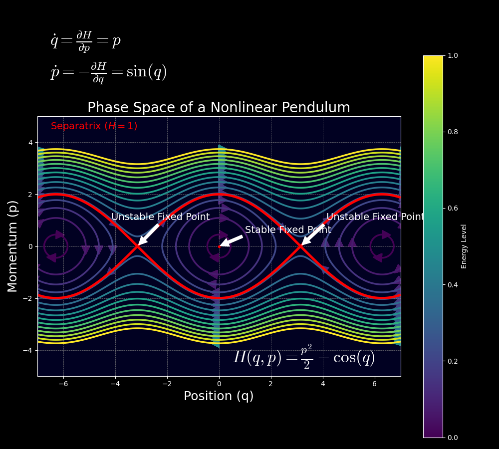
Interpreting the Pendulum's Phase Portrait:

• Closed Loops (inside the separatrix): These correspond to low energy states where the pendulum oscillates back and forth around the stable equilibrium at $\theta =0$. This motion is called libration. The trajectories are distorted ellipses, not perfect ellipses like the SHO, because the pendulum is a nonlinear oscillator.
• Wavy Lines (outside the separatrix): These are high energy states where the momentum is always large enough to carry the pendulum "over the top". This motion is called rotation. The pendulum continuously spins in one direction (either clockwise or counter-clockwise).
• The Separatrix: This is the critical curve (shown in red in the image above) that connects the unstable fixed points at $\theta =\pm \pi$. It corresponds to the exact energy required for the pendulum to start at the bottom and just barely reach the top, where it comes to rest momentarily. It separates the two distinct types of motion.

5. Advanced Example: Particle in a Cubic Potential

Let's apply our method to a problem you might encounter in a dynamics competition. Consider a particle of mass $m=1$ moving in a potential $V(x)=\frac{x^2}{2}-\frac{x^3}{3}$. (This is a slightly different potential from the one in the video, but the analysis is very similar).

The Hamiltonian is $H(x,p)=\frac{p^2}{2}+\frac{x^2}{2}-\frac{x^3}{3}$.
Hamilton's equations are $\dot{x}=p$ and $\dot{p}=-x+x^2$.

1. Fixed Points:

   • $\dot{x}=p=0$
   • $\dot{p}=-x+x^2=x(x-1)=0⟹x=0$ or $x=1$.
     We have two fixed points: $(x,p)=(0,0)$ and $(x,p)=(1,0)$.

2. Stability:

   • Near $x=0$, the potential $V(x)\approx x^2/2$, which is a minimum. This is a stable (elliptic) point.
   • Near $x=1$, the potential $V(x)$ has a maximum. This is an unstable (hyperbolic) point.

3. Global Portrait: We expect to see closed loops around $(0,0)$ and a saddle structure at $(1,0)$. The separatrix will emerge from the unstable point.

The following video walks through the complete construction of a very similar phase portrait. It uses a slightly different language (working with position $x$ and velocity $v$) but the method of finding fixed points and linearizing is precisely what we are doing. This is an excellent demonstration of the general applicability of these techniques in dynamical systems.

Conclusion

Today we transformed the abstract concept of phase space into a practical tool for analyzing physical systems. By constructing and interpreting phase portraits, we can gain deep, qualitative insights into the dynamics governed by a Hamiltonian.

Key Takeaways:

• For conservative systems, trajectories in phase space are the contour lines of the Hamiltonian $H(q,p)=E$.
• A systematic way to construct a phase portrait is to first find the fixed points ($\nabla H=0$) and then analyze their stability by linearizing the dynamics around them.
• Elliptic fixed points correspond to stable equilibria (potential minima) and are surrounded by closed orbits (oscillations).
• Hyperbolic fixed points correspond to unstable equilibria (potential maxima) and give rise to separatrices—special trajectories that divide the phase space into regions of qualitatively different motion.

Preview of the Next Lesson:
Our analysis today relied on linearizing Hamilton's equations around fixed points. This is a specific application of a much broader mathematical field: the theory of Ordinary Differential Equations (ODEs). In our next module, "Mathematical Methods for Physics," we will begin by formally learning how to solve the very types of first and second-order ODEs that arise in mechanics. The phase portraits you learned to draw today will serve as a powerful geometric guide to understanding the solutions you will soon learn to find analytically.