Solving Mechanics Problems with Euler-Lagrange Equations

Introduction

Welcome back! In our previous lesson, we mastered the crucial first step of the Lagrangian method: formulating the Lagrangian $L (q_{j}, q ˙_{j}, t)$ for a mechanical system using a well-chosen set of generalized coordinates $(q_{j})$ . We saw how this procedure elegantly incorporates constraints and simplifies the description of complex systems.

Today, we take the final, decisive step. We will take the Lagrangians we've constructed and substitute them into the Euler-Lagrange equations to derive the system's equations of motion. This lesson is where the formalism translates into concrete, predictive power. Our objective is to solve both unconstrained and constrained mechanics problems. We will first focus on the standard method where constraints are handled implicitly by the choice of coordinates. Then, we will introduce the powerful method of Lagrange multipliers to explicitly solve for the forces of constraint when needed.

1. The Euler-Lagrange Equations in Action

As we derived from the Principle of Stationary Action, the dynamics of any system are governed by the Euler-Lagrange equations. For a system with $n$ degrees of freedom described by generalized coordinates $q_{1}, \dots, q_{n}$ , there is one equation for each coordinate:

\frac{d}{d t} (\frac{\partial L}{\partial q ˙ _{j}}) - \frac{\partial L}{\partial q _{j}} = 0 for j = 1, \dots, n

The procedure is algorithmic:

For each generalized coordinate $q_{j}$ , compute the two partial derivatives:
- $\frac{\partial L}{\partial q _{j}}$ , the generalized force.
- $\frac{\partial L}{\partial q ˙ _{j}}$ , the generalized momentum, conjugate to $q_{j}$ .
Take the total time derivative of the generalized momentum: $\frac{d}{d t} (\frac{\partial L}{\partial q ˙ _{j}})$ .
Substitute these into the equation to get a second-order ordinary differential equation (ODE) for $q_{j} (t)$ .

Let's begin with a familiar case to see this in practice.

Example 1: The Simple Pendulum

In the last lesson, we derived the Lagrangian for a simple pendulum of mass $m$ and length $l$ :

L = \frac{1}{2} m l^{2} θ ˙^{2} + m g l cos θ

Here, we have one generalized coordinate, $q_{1} = θ$ . Let's apply the Euler-Lagrange equation:

Calculate derivatives:
- Generalized momentum $p_{θ} = \frac{\partial L}{\partial θ ˙} = m l^{2} θ ˙$ .
- Generalized force $F_{θ} = \frac{\partial L}{\partial θ} = - m g l sin θ$ .
Take time derivative of momentum:
- $\frac{d}{d t} (p_{θ}) = \frac{d}{d t} (m l^{2} θ ˙) = m l^{2} θ ¨$ .
Assemble the equation of motion:
$\frac{d}{d t} (\frac{\partial L}{\partial θ ˙}) - \frac{\partial L}{\partial θ} = 0$ $m l^{2} θ ¨ - (- m g l sin θ) = 0$ $m l^{2} θ ¨ + m g l sin θ = 0 ⟹ θ ¨ + \frac{g}{l} sin θ = 0$

This is the exact, non-linear equation of motion for a simple pendulum, which you have previously derived using Newtonian torque analysis. The Lagrangian method reproduces it with remarkable efficiency.

Example 2: Systems with Multiple Degrees of Freedom

The true power of this method becomes apparent in systems with multiple moving parts, where a Newtonian force analysis would be intricate. The following video demonstrates how to tackle a classic problem: a double pulley system with three masses.

Worked examples in classical Lagrangian mechanics

Let's apply this to a more complex system: the double pulley with three masses. This is a classic problem where Lagrangian mechanics shines. This video will walk us through the entire process, from setting up the two generalized coordinates to deriving the two coupled equations of motion.

Watch the segment from 13:56 to 26:55. Pay close attention to how the two generalized coordinates, q1 and q2, are defined. Follow the derivation of the kinetic and potential energies, leading to the full Lagrangian. The crucial part is seeing how the Euler-Lagrange equation is applied twice (once for q1, once for q2) to produce two distinct equations of motion.

As you saw, for a system with two degrees of freedom, we obtain two coupled second-order ODEs. Solving this system of equations provides the complete time evolution of the coordinates $q_{1} (t)$ and $q_{2} (t)$ .

2. Finding the Forces of Constraint

The standard Lagrangian method is designed to find the equations of motion without worrying about the forces that maintain the constraints (like tension or normal forces). But what if you need to find these forces? For this, we use the method of Lagrange Multipliers.

The core idea is to treat the system as less constrained than it is, and then add the constraint back in mathematically.

The Method:

Start with a coordinate system that has more degrees of freedom than the constrained system.
Write the constraint as an equation of the form $f (q_{1}, \dots, q_{k}) = 0$ .
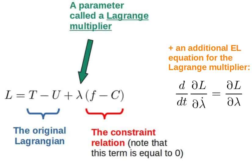
Construct an augmented Lagrangian, $L^{'}$ , by adding the constraint equation multiplied by a new variable, $λ$ (the Lagrange multiplier): $L^{'} = L (q_{j}, q ˙_{j}) + λ f (q_{j})$
Treat $λ$ as a new generalized coordinate. Now, derive the Euler-Lagrange equations for all original coordinates $q_{j}$ AND for $λ$ .
- The E-L equation for $λ$ is $\frac{\partial L ^{'}}{\partial λ} = 0$ , which simply returns the constraint equation $f (q_{j}) = 0$ .
- The E-L equations for the original coordinates $q_{j}$ become: $\frac{d}{d t} (\frac{\partial L}{\partial q ˙ _{j}}) - \frac{\partial L}{\partial q _{j}} = λ \frac{\partial f}{\partial q _{j}}$

The term on the right, $λ \frac{\partial f}{\partial q _{j}}$ , represents the generalized force of constraint corresponding to the coordinate $q_{j}$ . By solving the full system of equations, we can find both the motion and the value of $λ$ , which gives us the magnitude of the constraint force.

Lagrangian with Lagrange Multiplier for Constrained Systems — This image summarizes the method. The Lagrangian L is augmented by a term λf. We then treat λ as a coordinate, generating an extra Euler-Lagrange equation that enforces the constraint.

The following reading provides a rigorous but clear explanation of this method.

2. The Lagrangian Formalism

To understand the theory behind finding constraint forces, let's turn to David Tong's excellent lecture notes from Cambridge. This section introduces the method of Lagrange multipliers formally and shows how it allows us to solve for constraint forces by re-introducing the constraint equation into the Lagrangian.

Read Section 2.3, 'Constraints and Generalised Coordinates,' focusing on the material under the heading '2.3.1 Holonomic Constraints'. Follow the logic of creating the augmented Lagrangian L' and see how it is applied to the pendulum example to find the tension. This demonstrates how we get more information (the constraint force) at the cost of a slightly more complex calculation.

Example 3: Normal Force on a Particle on a Sphere

Let's find the normal force on a particle of mass $m$ sliding on the surface of a fixed, frictionless sphere of radius $R$ . We'll use spherical coordinates $r$ and $θ$ (measured from the vertical).

Coordinates and Constraint: We use two coordinates, $r$ and $θ$ . The constraint is that the particle stays on the sphere: $f (r) = r - R = 0$ .
Lagrangian: The Lagrangian for a free particle in a gravitational field in polar coordinates is:
$L = T - V = \frac{1}{2} m (r ˙^{2} + r^{2} θ ˙^{2}) - m g r cos θ$
The augmented Lagrangian is:
$L^{'} = \frac{1}{2} m (r ˙^{2} + r^{2} θ ˙^{2}) - m g r cos θ + λ (r - R)$
Euler-Lagrange Equations:
- For $λ$ : $\frac{\partial L ^{'}}{\partial λ} = r - R = 0$ , which is our constraint.
- For $θ$ :
  $\frac{d}{d t} (\frac{\partial L ^{'}}{\partial θ ˙}) - \frac{\partial L ^{'}}{\partial θ} = λ \frac{\partial f}{\partial θ}$
  $\frac{d}{d t} (m r^{2} θ ˙) - (- m g r sin θ) = λ (0)$
  $m r^{2} θ ¨ + 2 m r r ˙ θ ˙ + m g r sin θ = 0$
- For $r$ :
  $\frac{d}{d t} (\frac{\partial L ^{'}}{\partial r ˙}) - \frac{\partial L ^{'}}{\partial r} = λ \frac{\partial f}{\partial r}$
  $\frac{d}{d t} (m r ˙) - (m r θ ˙^{2} - m g cos θ + λ) = λ (1)$
  $m r ¨ - m r θ ˙^{2} + m g cos θ - λ = 0 ⟹ m r ¨ - m r θ ˙^{2} + m g cos θ = λ$
Solve for $λ$ : Now we apply the constraint $r = R$ , which implies $r ˙ = 0$ and $r ¨ = 0$ .
- The $θ$ equation becomes: $m R^{2} θ ¨ + m g R sin θ = 0 ⟹ θ ¨ = - \frac{g}{R} sin θ$ . This describes the motion.
- The $r$ equation becomes: $0 - m R θ ˙^{2} + m g cos θ = λ$ .

The generalized force of constraint is $λ \frac{\partial f}{\partial r} = λ$ . This is precisely the normal force $F_{N}$ . Therefore:

F_{N} = λ = m g cos θ - m R θ ˙^{2}

This result is exactly what you would find using Newton's second law in the radial direction ( $F_{n e t, r} = m a_{c}$ ), confirming the validity of the method.

Test your understanding!

Consider a simple Atwood's machine with masses $m_{1}$ and $m_{2}$ connected by a rope of length $l$ over a massless pulley. Let $x_{1}$ be the downward displacement of $m_{1}$ and $x_{2}$ be the downward displacement of $m_{2}$ , both measured from the pulley.

Use the method of Lagrange multipliers to find the tension $T$ in the rope.

(Hint: The unconstrained Lagrangian is for two separate falling masses. The constraint is $x_{1} + x_{2} = l$ .)

Show answer

Lagrangian and Constraint:
The kinetic energy is $T = \frac{1}{2} m_{1} x ˙_{1}^{2} + \frac{1}{2} m_{2} x ˙_{2}^{2}$ .
The potential energy is $V = - m_{1} g x_{1} - m_{2} g x_{2}$ .
The unconstrained Lagrangian is $L = T - V = \frac{1}{2} m_{1} x ˙_{1}^{2} + \frac{1}{2} m_{2} x ˙_{2}^{2} + m_{1} g x_{1} + m_{2} g x_{2}$ .
The constraint is $f (x_{1}, x_{2}) = x_{1} + x_{2} - l = 0$ .
Augmented Lagrangian:
$L^{'} = L + λ (x_{1} + x_{2} - l)$
Euler-Lagrange Equations:
- For $x_{1}$ :
  $\frac{d}{d t} (m_{1} x ˙_{1}) - (m_{1} g + λ) = 0 ⟹ m_{1} x ¨_{1} - m_{1} g = λ$
- For $x_{2}$ :
  $\frac{d}{d t} (m_{2} x ˙_{2}) - (m_{2} g + λ) = 0 ⟹ m_{2} x ¨_{2} - m_{2} g = λ$
Solve:
We have two equations:
(1) $m_{1} x ¨_{1} - m_{1} g = λ$
(2) $m_{2} x ¨_{2} - m_{2} g = λ$
From the constraint $x_{1} + x_{2} = l$ , we get $x ¨_{1} + x ¨_{2} = 0 ⟹ x ¨_{2} = - x ¨_{1}$ .
Substitute $x ¨_{2} = - x ¨_{1}$ into (2): $- m_{2} x ¨_{1} - m_{2} g = λ$ .
Now we have two expressions for $λ$ . Equating them:
$m_{1} x ¨_{1} - m_{1} g = - m_{2} x ¨_{1} - m_{2} g$
$x ¨_{1} (m_{1} + m_{2}) = g (m_{1} - m_{2}) ⟹ x ¨_{1} = g \frac{m _{1} - m _{2}}{m _{1} + m _{2}}$ . This is the familiar acceleration.

Now, substitute $x ¨_{1}$ back into equation (1) to find $λ$ :
$λ = m_{1} (g \frac{m _{1} - m _{2}}{m _{1} + m _{2}}) - m_{1} g = m_{1} g (\frac{m _{1} - m _{2} - ( m _{1} + m _{2} )}{m _{1} + m _{2}}) = m_{1} g (\frac{- 2 m _{2}}{m _{1} + m _{2}})$
$λ = - \frac{2 m _{1} m _{2} g}{m _{1} + m _{2}}$
The generalized constraint force for $x_{1}$ is $λ \frac{\partial f}{\partial x _{1}} = λ$ . This force acts in the direction of increasing $x_{1}$ (downward). The tension $T$ acts upward, so $T = - λ$ .
$T = \frac{2 m _{1} m _{2} g}{m _{1} + m _{2}}$
This is the well-known result for the tension in an Atwood's machine.

3. Engineering Application: Equilibrium in Rotating Systems

Lagrangian mechanics is exceptionally useful for analyzing stability in rotating systems, a common problem in mechanical engineering. Let's look at a bead on a spinning parabolic wire.

Worked examples in classical Lagrangian mechanics

To see these methods applied to a problem with an engineering flavor, let's analyze a bead on a rotating parabolic wire. This problem involves a time-dependent constraint and allows us to investigate equilibrium conditions in a rotating frame, a common task in mechanical engineering.

Watch the segment from 53:53 to 1:06:09. Observe how the Lagrangian is constructed using cylindrical coordinates but with constraints applied (z as a function of r, and θ as a function of t). The most interesting part is the derivation of the equation of motion for 'r' and the subsequent analysis to find the equilibrium conditions. This shows how we can use the E-L equations not just for dynamics, but also for finding stable/unstable configurations.

This example shows how the derived equation of motion, even if complex, can be immediately used to analyze important physical properties like equilibrium points by setting velocities and accelerations to zero.

Conclusion

In this lesson, you have learned to wield the full power of the Euler-Lagrange equations. You can now take a physical system, construct its Lagrangian, and derive the differential equations that completely govern its motion.

Key Takeaways:

The Euler-Lagrange equation $\frac{d}{d t} (\frac{\partial L}{\partial q ˙ _{j}}) - \frac{\partial L}{\partial q _{j}} = 0$ provides a systematic, algorithmic way to find the equations of motion for any system described by a Lagrangian.
For a system with $n$ degrees of freedom, this method yields $n$ second-order ODEs.
The standard method is ideal for finding the system's trajectory, as it conveniently eliminates constraint forces.
When constraint forces themselves are of interest, the method of Lagrange multipliers allows us to find them by augmenting the Lagrangian and treating the multiplier $λ$ as an additional coordinate. The value of $λ$ is directly related to the magnitude of the constraint force.

Preview of the Next Lesson:
In several examples today (like the spherical pendulum or the particle on a cone), you may have noticed that the Lagrangian did not depend on an angle coordinate (e.g., $ϕ$ ), but only on its velocity ( $ϕ ˙$ ). Such coordinates are called cyclic or ignorable. In our next lesson, we will explore the profound consequence of this observation: whenever a coordinate is cyclic, its corresponding generalized momentum is conserved. This is a direct manifestation of Noether's Theorem, which connects symmetries in the Lagrangian to conserved quantities in the system.

Recommended resources