Lagrangian Formulation with Generalized Coordinates

1. From Cartesian Coordinates to Generalized Coordinates

The primary motivation for moving beyond Cartesian coordinates is to simplify the description of a system. For a simple pendulum, describing the motion with $x$ and $y$ is clumsy because you also need to enforce the constraint $x^2+y^2=l^2$. It's far more natural to use a single angle, $\theta$. This angle is an example of a generalized coordinate.

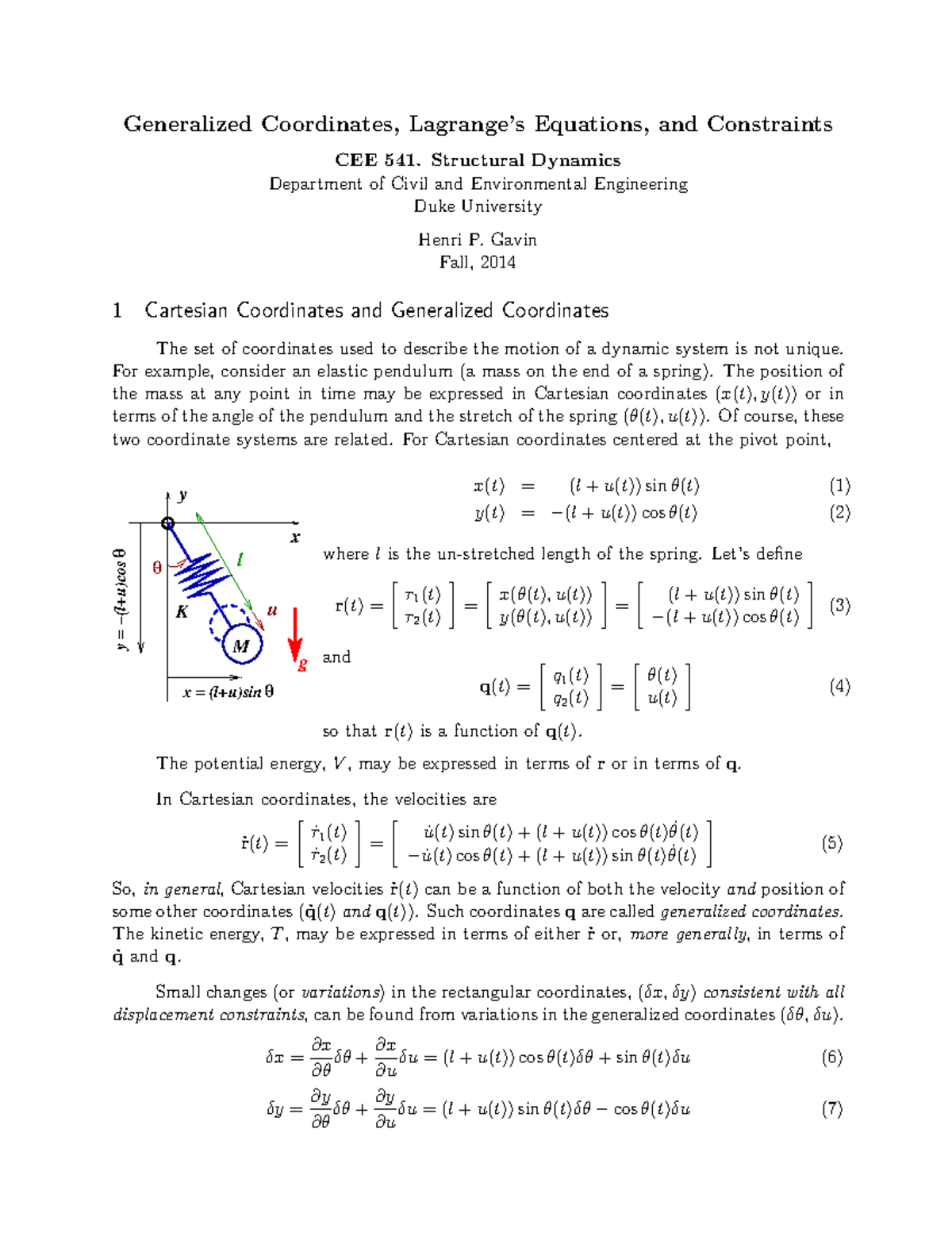
To formalize this, we need two key concepts:

1. Degrees of Freedom (DoF): The number of independent variables required to completely specify the configuration of a system. A free particle in 3D has 3 DoF. A rigid dumbbell in 3D has 5 DoF (3 for position of center of mass, 2 for orientation).
2. Constraints: Physical limitations on the motion of a system. A bead on a wire is constrained to move along the wire. A pendulum bob is constrained to maintain a fixed distance from its pivot. Each holonomic constraint (a constraint expressible as an algebraic equation relating coordinates, e.g., $x^2+y^2-l^2=0$) reduces the number of DoF by one.

Generalized Coordinates, denoted $q_1,q_2,\dots ,q_n$, are a set of $n$ independent variables, where $n$ is the number of DoF, that uniquely defines the state of the system. They can be lengths, angles, or any other convenient quantity.

The following video provides a rigorous discussion of these concepts, including how to determine the number of DoF for various systems.

2. The Procedure for Formulating the Lagrangian

Now that we understand the concept of generalized coordinates, we can establish a universal recipe for writing down the Lagrangian of any mechanical system.

The General Steps:

1. Analyze the System: Determine the number of particles (N) and identify all holonomic constraints (k). Calculate the number of degrees of freedom: $n=3N-k$ (for 3D motion).
2. Choose Generalized Coordinates: Select a set of $n$ independent coordinates $q_1,q_2,\dots ,q_n$ that conveniently describe the system's configuration.
3. Express Cartesian Positions: Write the Cartesian coordinates $(x,y,z)$ of each particle in the system as functions of your chosen generalized coordinates and time: $x_i=x_i(q_1,\dots ,q_n,t)$, etc.
4. Find Cartesian Velocities: Differentiate the position expressions with respect to time to find the velocity components $({\dot{x}}_i,{\dot{y}}_i,{\dot{z}}_i)$ in terms of the generalized coordinates and their time derivatives $(q_j,{\dot{q}}_j,t)$. This step usually involves the chain rule.
5. Calculate Kinetic Energy (T): Form the total kinetic energy $T={\sum }_i\frac{1}{2}{m}_i({\dot{x}}_i^2+{\dot{y}}_i^2+{\dot{z}}_i^2)$. Substitute the velocity expressions from Step 4. The result will be $T(q_j,{\dot{q}}_j,t)$.
6. Calculate Potential Energy (V): Form the total potential energy $V$. Substitute the position expressions from Step 3. The result will be $V(q_j,t)$.
7. Construct the Lagrangian: The Lagrangian is simply $L=T-V$.

Let's illustrate this with the classic simple pendulum.

• Step 1: 1 particle, 2 constraints (motion in a plane, say $z=0$, and fixed length $x^2+y^2=l^2$). DoF = 3(1) - 2 = 1.
• Step 2: Choose one generalized coordinate, the angle $\theta$.
• Step 3: Let the pivot be at the origin. $x=l\sin \theta$, $y=-l\cos \theta$.
• Step 4: $\dot{x}=l\dot{\theta }\cos \theta$, $\dot{y}=l\dot{\theta }\sin \theta$.
• Step 5: $T=\frac{1}{2}m({\dot{x}}^2+{\dot{y}}^2)=\frac{1}{2}m(l^2{\dot{\theta }}^2{\cos }^2\theta +l^2{\dot{\theta }}^2{\sin }^2\theta )=\frac{1}{2}m{l}^2{\dot{\theta }}^2$.
• Step 6: Using the pivot as the zero potential level, $V=mgy=-mgl\cos \theta$.
• Step 7: $L=T-V=\frac{1}{2}m{l}^2{\dot{\theta }}^2+mgl\cos \theta$.

This is the Lagrangian for a simple pendulum. Notice how the constraints are automatically satisfied by our choice of coordinate, and we are left with a simple expression involving only one variable. The following resource provides several more clean examples.

3. A Complete Worked Example: The Cylindrical Pendulum

The procedure works just as well for more complex systems involving both translation and rotation. Let's walk through a complete derivation for a rigid cylinder suspended by a string, which can swing like a pendulum and also rotate about its own axis.

This video breaks down the process meticulously, from choosing coordinates to deriving the final Lagrangian.

Conclusion

Today, we've taken the abstract formalism of the Euler-Lagrange equation and turned it into a concrete, powerful tool for analyzing physical systems. You now have a systematic method to tackle complex mechanics problems that might be intractable using Newtonian force analysis.

Key Takeaways:

• Generalized Coordinates ($q_i$) are any set of independent variables, equal in number to the system's degrees of freedom, that uniquely specify its configuration.
• The choice of coordinates is flexible; we choose them to simplify the problem and automatically satisfy constraints.
• We have a 7-step procedure to derive the Lagrangian $L=T-V$: choose coordinates, write Cartesian positions in terms of them, find velocities, and then assemble the kinetic and potential energies.
• The resulting Lagrangian, $L(q_j,{\dot{q}}_j,t)$, is a scalar function that contains all the dynamical information of the system.

Preview of the Next Lesson:
We have successfully mastered the art of formulating the Lagrangian. The next logical step is to use it. In our next lesson, we will take the Lagrangians we've learned to construct, plug them into the Euler-Lagrange equation $\frac{d}{dt}\left(\frac{\partial L}{\partial {\dot{q}}_j}\right)-\frac{\partial L}{\partial q_j}=0$, and derive the full equations of motion for these systems. This is where we will see the elegant mathematics translate into concrete predictions about how systems evolve in time.