In our previous lesson, we mastered static formatting, learning to control the appearance of cells with custom number formats and reusable cell styles. This gave us the power to create polished, professional reports. Now, we'll take the next logical step and make our formatting dynamic.
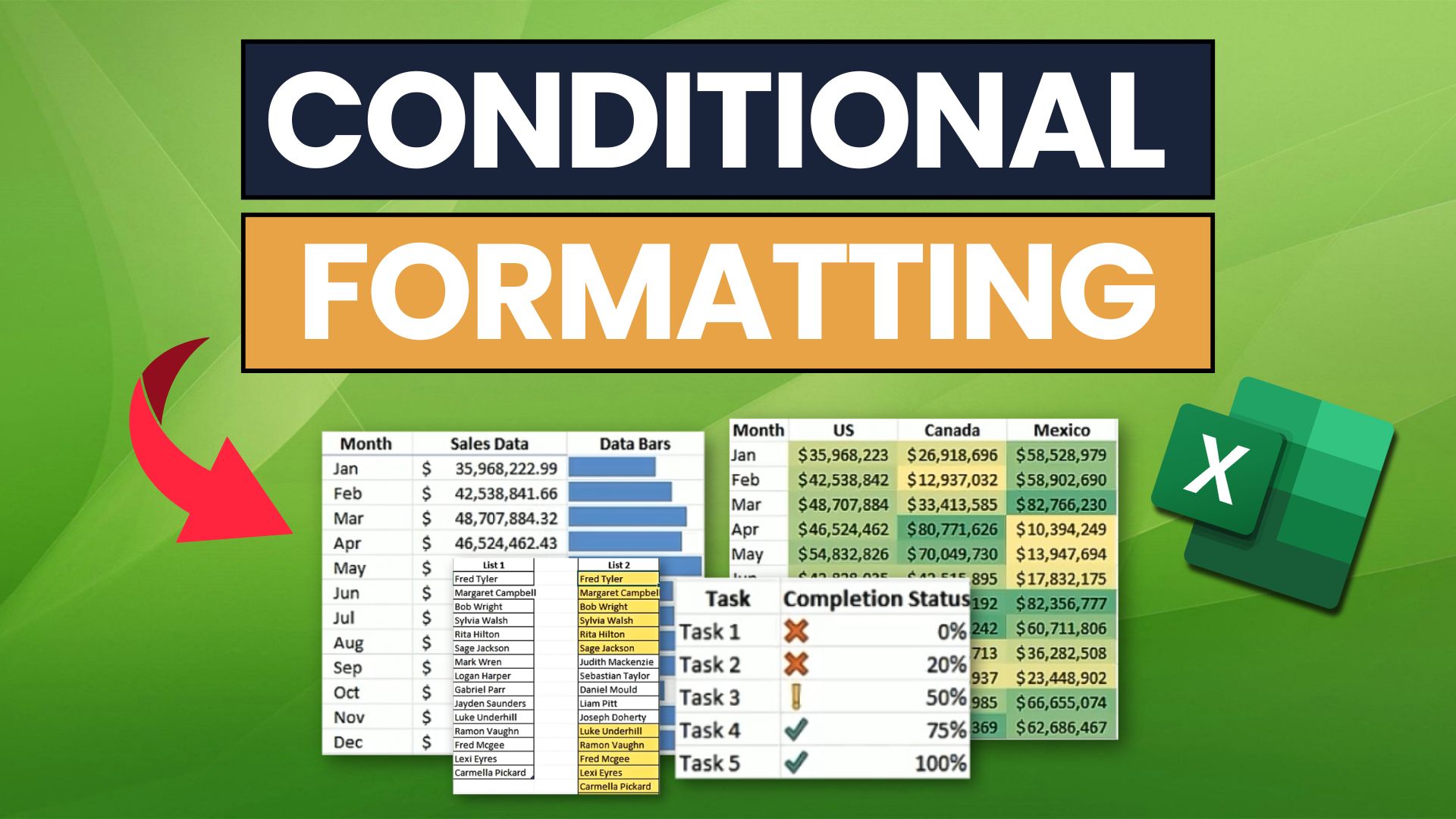
This lesson introduces Conditional Formatting, one of Excel's most powerful features for data analysis and presentation. Instead of manually coloring cells, you'll create rules that automatically format them based on their values. This allows you to instantly spot trends, identify outliers, and highlight critical information in your data. For a freelancer, this skill is essential for building intuitive dashboards and client-ready reports that tell a clear story.
Our focus will be on applying Excel's versatile set of built-in or "preset" rules, specifically:
- Highlighting cells that meet certain criteria (e.g., greater than a specific value).
- Pinpointing top or bottom performers.
- Using in-cell graphics like Data Bars, Color Scales, and Icon Sets to visualize data.
Rule-Based Highlighting
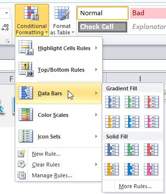
The fundamental principle of conditional formatting is straightforward: you select the data you want to format, choose a rule from the Home > Conditional Formatting menu, and define the criteria. Let's start with the most common types: Highlight Cells Rules and Top/Bottom Rules.
These rules are perfect for tasks like identifying sales figures below a target, flagging overdue dates, or finding duplicate entries in a client list.
The video below by Kevin Stratvert provides a clear, practical introduction to applying a basic highlighting rule.
Conditional Formatting in Excel Tutorial
This video demonstrates the core concept of applying a conditional formatting rule to highlight cells that meet a specific numerical condition.
Please watch the segment on highlighting scores. Notice how quickly the formatting allows you to identify the data points of interest.
Applying a rule is easy, but the real power comes from customizing it. You are not limited to the default options. You can edit any rule to change its logic or its appearance.
The next video, from Kenji Explains, demonstrates how to apply a rule and then modify it to fit a more specific need—a crucial skill for professional work.
Master Conditional Formatting in Excel (The CORRECT Way)
This video shows how to apply a 'Greater Than' rule and then edit it to be 'Greater Than or Equal To', as well as how to apply a completely custom fill color.
Watch the segment from the beginning. Pay close attention to how he accesses the Manage Rules dialog to edit the existing rule. This dialog is the central hub for all conditional formatting in a sheet.
Excel offers a rich library of preset rules. Beyond simple numerical comparisons, you can highlight top or bottom values, dates, and even duplicate or unique text. Let's look at a few more common examples.
Conditional Formatting in Excel Tutorial
Continuing with Kevin Stratvert's tutorial, these clips show how to handle dates and find duplicates.
Watch the following segments: Formatting by date: See how to highlight recent entries, a useful technique for tracking new data. Finding duplicates: This is an invaluable tool for data cleaning, a common task for any data professional.
In-Cell Data Visualization
While highlighting cells is useful, conditional formatting can also turn your cells into miniature data visualizations. This helps you and your clients compare values across a large dataset without having to build a separate chart. The three primary tools for this are Data Bars, Color Scales, and Icon Sets.
Data Bars
Data Bars place a small bar chart directly inside each cell. The length of the bar is proportional to the cell's value relative to the other selected cells. This is an incredibly effective way to see the magnitude of numbers at a glance.
Master Conditional Formatting in Excel (The CORRECT Way)
This segment from Kenji Explains demonstrates the application of Data Bars and explains why they are often a better choice than Color Scales for comparing values.
Please watch from this section on Data Bars. Note how much easier it is to compare the sales figures with the bars versus just looking at the numbers alone.
Color Scales
Color Scales apply a color gradient across a range of cells. For example, you can have a scale that goes from red (lowest values) to yellow (mid-range values) to green (highest values), creating a "heat map" effect. This is useful for visualizing the distribution and variation in a large dataset, such as monthly temperatures or survey results.
Conditional Formatting in Excel Tutorial
This short clip gives a quick demonstration of how Color Scales look when applied to a set of student scores.
Watch this brief segment on Color Scales to see them in action.
Icon Sets
Icon Sets classify your data into categories by placing an icon in each cell. Common sets include traffic lights (red, yellow, green) or trend arrows (up, down, sideways). This is a great way to communicate status or performance (e.g., project on track, at risk, or delayed).
A critical professional habit is to always check the logic behind an icon set. By default, Excel often applies icons based on percentages (e.g., top 33% get a green icon). This can be misleading. You should almost always edit the rule to use specific number thresholds that make sense for your data.
Master Conditional Formatting in Excel (The CORRECT Way)
This is one of the most important parts of the lesson. The video demonstrates why the default icon set rule is flawed and how to fix it by changing the rule's logic from 'Percent' to 'Number'.
Watch carefully from this section on Icon Sets. Understanding how to customize this logic is a key step toward using conditional formatting accurately and professionally.
Applying and Managing Rules: A Quick Reference
You've now seen how to apply the most common built-in conditional formatting rules. For a comprehensive and practical reference, the official Microsoft Support documentation provides clear, step-by-step instructions. The following reading gives concise summaries for applying Data Bars, Color Scales, and Icon Sets.
Use conditional formatting to highlight information in Excel
This article from Microsoft Support serves as an excellent quick reference guide. We will focus on the clear, step-by-step instructions for the visual formatting types.
Please review the following short sections: Read the section on Data Bars. Next, review the two sections under Color Scales. Finally, read the section on Icon Sets.
Conclusion
In this lesson, you've moved from static to dynamic formatting, a major step in your journey to becoming an Excel expert. You now have the tools to make your data speak for itself, automatically highlighting key insights and visualizing trends without manual effort.
Key Takeaways:
- Conditional Formatting is Dynamic: It applies formatting based on rules that automatically update when your data changes.
- Built-in Rules are Powerful:
Highlight Cells RulesandTop/Bottom Rulesoffer quick ways to flag important data points like values over a certain threshold, dates, or duplicates. - In-Cell Visuals Aid Analysis: Data Bars, Color Scales, and Icon Sets turn your data range into a visual dashboard, making it easy to compare values and spot patterns.
- Customization is Key: For professional results, always review the logic of a conditional formatting rule—especially for Icon Sets—and adjust it to use specific numbers or conditions that accurately reflect your data's meaning. All rules can be reviewed and edited from the
Conditional Formatting > Manage Rulesdialog.
So far, we've relied on Excel's built-in rules. But what if your condition is more complex? For example, what if you need to highlight an entire row based on the value in a single cell in that row? To do that, you need to write your own rules using formulas. That is precisely the topic of our next lesson.