Introduction
In our last lesson, we explored Excel's powerful built-in conditional formatting rules, learning to make our data dynamic by applying formatting like Data Bars, Color Scales, and various presets. While these tools are excellent for many situations, their logic is predefined. To truly unlock the full potential of conditional formatting and build the sophisticated, custom reports your future clients will demand, you need to write your own rules.
This lesson bridges that gap. We will move beyond presets and learn how to create custom conditional formatting rules using formulas. This gives you complete control, allowing you to apply formatting based on complex criteria that Excel's built-in rules can't handle. We'll focus on the core principles, the critical role of cell references, and practical techniques for highlighting information, such as formatting an entire row based on the value in a single cell.
1. The Core Principle: A Formula Must Return TRUE or FALSE
The entire system of formula-based conditional formatting rests on one simple idea: Excel applies the format only if your formula evaluates to TRUE. If the formula returns FALSE, zero, or an error, the format is not applied.
The video below explains this fundamental concept, which is the first "simple rule" to mastering this feature.
Conditional Formatting Formulas - Mystery Solved with 3 Simple Rules
This clip from MyOnlineTrainingHub breaks down the foundational logic of conditional formatting formulas.
Watch the segment explaining the first rule. The key takeaway is that your formula must produce a logical TRUE or FALSE result. Note that Excel also treats any non-zero number as TRUE.
Formulas that use comparison operators (e.g., =A1>100) or logical functions (e.g., =ISNUMBER(A1), =AND(B2="Shipped", C2>50)) are perfect for this, as they are designed to return TRUE or FALSE.
2. The Process: Creating Your First Formula-Based Rule
Now that you understand the underlying logic, let's walk through the mechanical steps of creating a rule. The process is consistent: you select the cells you want to format, open the "New Rule" dialog, and input your custom formula.
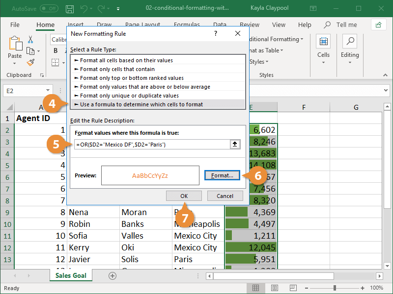
The following reading provides a clear, step-by-step guide to this process.
Excel conditional formatting formulas based on another cell
This section from a comprehensive article by Ablebits.com details the exact steps to create a formula-based rule.
Please read the section titled "How to create a rule". Focus on the sequence of actions, from selecting your data range to choosing the formula option and setting the format.
3. The Key to Control: Understanding Cell References
This is the most critical and often trickiest part of using formulas in conditional formatting. When you write a formula, you must write it from the perspective of the top-left cell in your selected range. Excel then "virtually" applies that formula to every other cell in the selection, automatically adjusting any relative cell references.
This is where your knowledge of absolute ($A$1), relative (A1), and mixed ($A1 or A$1) references from our first module becomes essential. Getting the references right is the difference between formatting a single cell and formatting an entire row based on a condition.
- To check a value in the same column but different rows, use a mixed reference that locks the column but keeps the row relative (e.g.,
$B2). - To check a value against a single, fixed cell (like a sales target in cell F1), use an absolute reference (e.g.,
$F$1).
The following video brilliantly demonstrates this concept, showing first how to format individual cells and then how to adjust the formula to format entire rows.
Excel Conditional Formatting with Formula | Highlight Rows based on a cell value
This tutorial from Leila Gharani provides an exceptionally clear explanation of how cell references work in conditional formatting.
Watch these two crucial segments: Start with the section on highlighting individual cells. Pay close attention to how she first gets the wrong result with absolute references ($B$6) and then corrects it by making the row reference relative (B6). Next, watch the segment on highlighting entire rows. This is the most important part. Notice how she uses the mixed reference =$F6 to ensure that every cell in a given row always refers back to the value in column F for that same row.
4. A Practical Habit: Test Your Formulas on the Grid
You cannot debug formulas inside the conditional formatting manager. If a rule doesn't work, Excel gives you no feedback. To avoid frustration, adopt the professional habit of testing your formula directly on the worksheet in a temporary "helper column."
The idea is simple:
- Next to your data, pick an empty column.
- In the first row of that column (level with your data), type the exact formula you plan to use for your conditional formatting.
- Drag the formula down.
- You will now see a column of
TRUEandFALSEvalues. This shows you exactly which rows your conditional formatting rule will format. If the results are what you expect, you can confidently copy the formula from the first cell, delete the helper column, and paste the formula into the rule manager.
The video you just watched introduced this technique. The reading below, from Exceljet, reinforces it under the name "Dummy Formulas."
Conditional formatting with formulas
This resource explains the value of testing your formulas directly on the worksheet to visualize their results before applying them as a rule.
Read the section from Troubleshooting and Dummy Formulas. This will solidify the testing technique we've discussed.
5. Putting It All Together: Common Scenarios
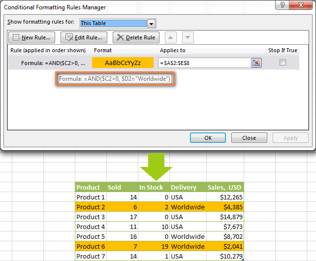
Let's look at a common business scenario: highlighting rows that meet multiple criteria. For this, we use the AND function, which returns TRUE only if all of its conditions are met.
Imagine you have a sales table and you want to highlight rows where the "In Stock" column is greater than 0 AND the "Delivery" column is "Worldwide". The formula, written for row 2, would be: =AND($C2>0, $D2="Worldwide")
- The
$locks the columns, so even when formatting cells in columns A, B, or E, the formula still checks columns C and D. - The row number
2is relative, so it updates to3,4,5, etc., as Excel evaluates the rule for each subsequent row.
The image below shows the result of exactly this type of formula.
The Ablebits.com article provides an excellent library of formulas for various scenarios. You don't need to memorize them, but it's good to know what's possible.
Excel conditional formatting formulas based on another cell
This article provides a rich set of practical formulas you can adapt for your own use.
Skim through the section "Formula examples". Pay particular attention to the tables showing formulas for comparison, AND/OR logic, and working with text values. This is a great resource to bookmark for future reference.
If your rule isn't behaving, the troubleshooting guide in the same article is an invaluable checklist.
Excel conditional formatting formulas based on another cell
This section provides a checklist of the most common reasons a conditional formatting rule fails.
Read the section titled "Why isn't my conditional formatting working?". Internalizing these checks will save you significant time when building reports.
Conclusion
You have now moved from a user of conditional formatting to an architect of it. By mastering the use of formulas, you can create formatting rules that are precisely tailored to any analytical need, resulting in clearer, more insightful, and more professional reports.
Key Takeaways:
- The TRUE/FALSE Rule: A conditional formatting formula must evaluate to
TRUE(or a non-zero number) for the format to be applied. - Write for the Top-Left Cell: Your formula should be written as if it's for the top-left cell of your selected range.
- Master Mixed References: Using mixed references (e.g.,
$A1) is the key to formatting entire rows based on a condition in a specific column. - Test on the Grid: Always test your formulas in a helper column to see the
TRUE/FALSEoutputs before creating the rule. This is the most effective way to debug. - Combine Functions for Power: Use functions like
ANDandORto build rules based on multiple criteria.
In our next lesson, we will apply these presentation skills as we learn to design and build reusable spreadsheet templates. The dynamic highlighting you've learned today is a cornerstone of creating professional, intuitive tools for yourself and your clients.