Introduction
Welcome to the next lesson in our journey through financial modeling. In previous sessions, we explored the time value of money using functions like PV, FV, and PMT to get single-value answers for loans and investments. Last time, we elevated this by using NPV and IRR to evaluate the entire lifecycle of a project. Today, we'll apply these skills to a very common and practical task for any financial analyst: building a detailed loan amortization schedule.
A loan amortization schedule provides a period-by-period breakdown of a loan, showing exactly how much of each payment goes toward interest versus how much goes toward paying down the principal. This lesson will guide you through creating a dynamic and reusable amortization schedule in Excel. This is not just a theoretical exercise; it’s a tangible tool you can build and adapt for future freelance clients who need to understand the true cost and progression of their loans.
1. The Structure of an Amortization Schedule
Before we dive into formulas, let's establish the components of a standard amortization schedule. It typically consists of two parts:
-
Input Section: This is where we define the core parameters of the loan. It's best practice to keep these inputs separate so they can be easily changed.
- Loan Amount (the principal, )
- Annual Interest Rate
- Loan Term (usually in years)
- Payments Per Year (e.g., 12 for monthly)
-
Schedule Table: This is the detailed breakdown of each payment over the life of the loan.
- Period: The payment number (1, 2, 3, ...).
- Payment: The fixed periodic payment amount, which we can calculate with the
PMTfunction. - Interest: The portion of the payment that covers the interest accrued during that period.
- Principal: The portion of the payment that reduces the outstanding loan balance.
- Remaining Balance: The outstanding loan amount after the payment is made.
Here is an example of a completed amortization schedule. This is what we will build today.

2. Calculating the Core Components
The first step is to calculate the fixed monthly payment. As we've seen before, the PMT function is perfect for this. The key is to ensure the rate and number of periods match the payment frequency (e.g., monthly).
- Rate: Annual Interest Rate / Payments Per Year
- Nper: Loan Term (in years) * Payments Per Year
- Pv: The loan amount
The formula will look like this: =PMT(rate, nper, pv). When building the schedule, it's crucial to use absolute references (e.g., $C$2) for the inputs, so the formulas can be dragged down without the references changing.
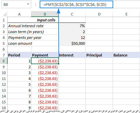
Once you have the fixed payment, the logic for each row of the schedule is as follows:
- Beginning Balance: For the first period, this is the total loan amount. For all subsequent periods, it's the ending balance from the previous period.
- Interest Paid: This is calculated on the beginning balance for the current period. The formula is:
Beginning Balance * (Annual Interest Rate / Payments Per Year). - Principal Paid: This is the remainder of your fixed payment after the interest has been paid. The formula is simply:
Payment - Interest. - Ending Balance: This is the beginning balance less the principal portion you just paid off. The formula is:
Beginning Balance - Principal.
This cycle repeats until the ending balance reaches zero.
3. Building the Schedule: A Step-by-Step Guide
The following video provides an excellent, clear walkthrough of creating a schedule from scratch using the logic we just discussed. It also demonstrates the critical importance of using absolute and relative cell references correctly.
How To Create an Amortization Table In Excel
This video from The Organic Chemistry Tutor will guide you through the entire process of building a functional amortization table.
Please watch the following segments carefully: Initial setup: See how to organize the input cells and calculate the monthly payment using PMT. First row calculation: Follow the logic for calculating the interest, principal, and ending balance for the very first payment. Extending the formulas: This is a crucial section. Pay close attention to how absolute references ($) are used to "lock" the references to the input cells, while relative references are used for values within the schedule itself. This is what allows you to automate the entire table by dragging the formulas down. Finishing the table: Watch how to extend the schedule to the final payment and verify that the ending balance correctly goes to zero.
4. An Alternative Method: IPMT and PPMT Functions
The method shown in the video is fantastic because it builds the logic from first principles. However, Excel also has specialized functions that can calculate the interest and principal portions of a payment directly: IPMT and PPMT.
=IPMT(rate, per, nper, pv): Calculates the interest portion for a specific period.=PPMT(rate, per, nper, pv): Calculates the principal portion for a specific period.
The arguments are almost identical to the PMT function, with one important addition:
- per: This is the specific period for which you want to calculate the interest or principal. This argument should be a relative reference to the "Period" column in your schedule.
This reading from Ablebits.com provides a great tutorial on using these functions to build your schedule.
Create a loan amortization schedule in Excel (with extra ...
This article provides a step-by-step guide to building a schedule using the IPMT and PPMT functions.
Please read the first five sections, from the beginning down to the end of section 5. Focus on the syntax for the PMT, IPMT, and PPMT functions. Notice how the per argument in IPMT and PPMT is a relative reference to the period number in column A, allowing the formula to calculate the correct amount for each specific row.
At any given period, the sum of the IPMT and PPMT results will equal the result of the PMT function. This provides a useful way to check your work.
5. Creating a Reusable, Dynamic Tool
A good financial tool is robust and flexible. The schedules we've built so far work perfectly, but what if a client wants to see the schedule for a 15-year loan instead of a 30-year loan? The table would show error messages or incorrect values beyond the 180th payment.
To build a truly professional template, we can wrap our formulas in an IF statement. The logic is simple: "If the current period number is within the loan term, perform the calculation; otherwise, show a blank cell."
The formula structure looks like this:=IF(current_period_number <= total_number_of_periods, [your_formula], "")
The following video from the Corporate Finance Institute demonstrates this technique effectively, turning a static schedule into a dynamic tool.
How to Create a Debt Schedule in Excel with PMT, IPMT & IF Functions
This video demonstrates how to use an IF statement to make your amortization schedule dynamic.
Watch the section from incorporating an IF statement. The key takeaway is seeing how wrapping the PMT and IPMT formulas inside an IF function allows the schedule to adjust automatically when you change the loan term. This prevents errors and makes the tool far more user-friendly.
This technique is fundamental to building high-quality, reusable templates for clients.
Conclusion
In this lesson, you have moved from calculating single-value loan metrics to building a comprehensive, period-by-period schedule. This is a significant step toward creating sophisticated financial models.
Key Takeaways:
- An amortization schedule breaks down each loan payment into its interest and principal components.
- The core logic is that interest is calculated on the outstanding balance, and the rest of the payment reduces that balance.
- You can calculate the principal and interest breakdown manually (
Payment - Interest) or by using Excel's dedicatedIPMTandPPMTfunctions. - Correctly using absolute (
$A$1) and relative (A1) cell references is essential for automating the schedule creation. - Wrapping formulas in an
IFstatement makes your schedule dynamic and robust, turning it into a professional, reusable tool.
In our next lesson, we will leverage the dynamic schedule we've just built to perform sensitivity analysis. We will use Excel's Data Tables to explore how changes in key assumptions, like the interest rate or loan term, impact the monthly payment and total interest paid.