Interactive Chart Controls

Introduction

In our last lesson, you learned how to add Slicers and Timelines to create interactive dashboards, which are fantastic for filtering data by different categories. We're now going to explore a different, and in many ways more powerful, type of interactivity using form controls. While slicers let users filter existing data, form controls can fundamentally change what a chart displays—for example, allowing a user to switch a chart from showing "Total Sales" to "Profit Margin" with a single click.

This lesson directly addresses the learning outcome of incorporating form controls like drop-down lists to create interactive chart inputs. Mastering this will add a significant tool to your freelance arsenal, enabling you to build highly dynamic and client-friendly reports. We will cover how to insert these controls, link them to your worksheet, and use formulas to make your charts respond to user selections.

1. Understanding Form Controls

Form controls are objects you can place on your worksheet to allow for user interaction without needing to write any VBA code (at least for now). They are found on the Developer tab in the Excel ribbon. If you don't see this tab, you can enable it by right-clicking the ribbon, selecting "Customize the Ribbon...", and checking the "Developer" box.

These controls include buttons, checkboxes, option buttons (also called radio buttons), and combo boxes (drop-down lists).

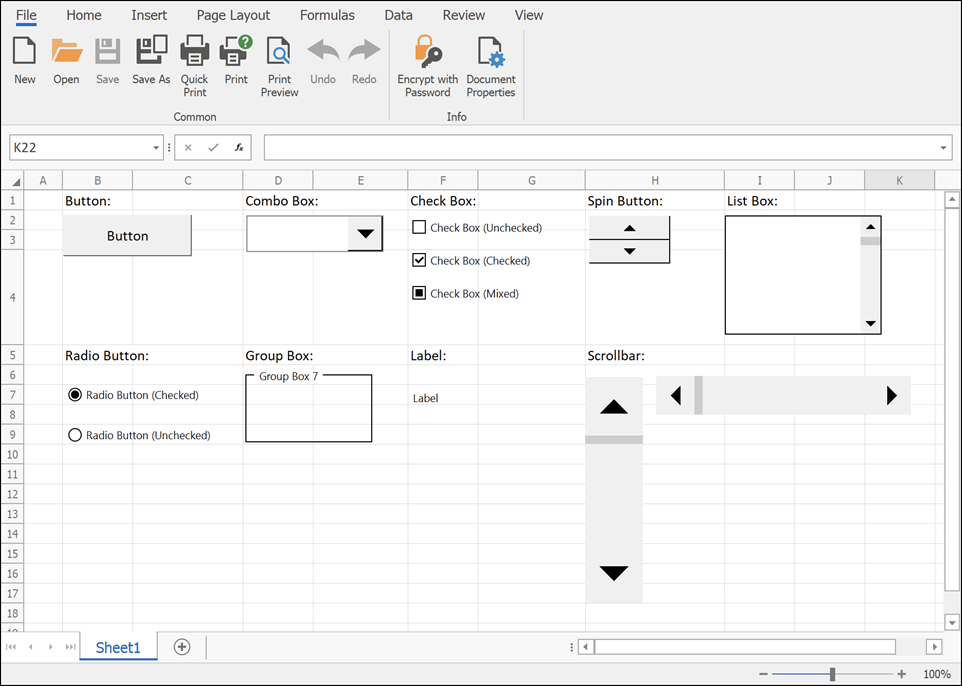
This image shows several of the form controls available in Excel, such as buttons, checkboxes, and combo boxes. We will focus on the most useful ones for building interactive charts.

The core principle behind using form controls is a three-step process:

Insert the control onto your worksheet.
Link the control to a specific cell. The control's state (e.g., which option is selected, whether a box is checked) will output a value into this linked cell.
Use the value in the linked cell to drive formulas that dynamically prepare the data that your chart is based on.

Let's see this in action, starting with Option Buttons.

2. Selecting a Metric with Option Buttons

Option buttons are ideal when you want a user to choose one exclusive option from a small set of choices (e.g., "Game," "Productivity," or "Utility"). When you click one option, the others are automatically deselected.

The following video provides an excellent, modern approach to using option buttons to create a dynamic chart. Pay close attention not just to inserting the buttons, but to the formulas used to make the data respond.

Create INTERACTIVE Excel Dashboards With Option Buttons | How to use Radio Buttons

The video "Create INTERACTIVE Excel Dashboards With Option Buttons" from the Leila Gharani channel demonstrates the complete process, from adding the controls to creating a dynamic data source with modern Excel functions.

First, watch how to insert and link option buttons. Notice how selecting an option button places a number (1, 2, or 3) into the single linked cell. This number is the key to our interactivity. Next, see how this linked number is used to create a dynamic data source. The video explains how to use the SWITCH function to translate the number (1) into the corresponding text ("Game") and then use that text inside a FILTER function to extract the relevant data. This is a powerful and flexible technique.

By completing these steps, you create a system where clicking an option button changes the number in the linked cell, which in turn causes the SWITCH and FILTER formulas to recalculate, producing a new set of data for your chart.

3. Using a Combo Box for Longer Lists

Option buttons are great for 2-4 choices, but they take up a lot of space. For longer lists of selectable metrics or categories, a Combo Box (a drop-down list) is a more compact and professional choice.

The setup is slightly different. Instead of just a linked cell, you also need to specify an "Input range"—the list of text options that will appear in the drop-down.

The Format Control settings are the heart of a form control's functionality. For a Combo Box, the 'Input range' defines the list of items in the drop-down, and the 'Cell link' specifies where the numeric result of the user's selection will be placed.

The TrumpExcel video below gives a clear walkthrough of setting up a Combo Box.

Excel Dashboard Course #10 - Excel Interactive Controls (Scrollbar, Spin Button, Checkbox, Combobox)

This video, "Excel Interactive Controls," provides a clear demonstration of setting up and using a Combo Box.

First, watch the segment on setting up the Combo Box. Pay attention to how the Input range and Cell link are configured in the "Format Control" dialog. Then, watch how the linked cell's output is used with an INDEX formula to pull the correct data for the chart. While this video uses the INDEX function, you could just as easily use the SWITCH and FILTER technique you learned in the previous section. The principle is the same: the Combo Box outputs a number, and that number drives your formulas. 4. Advanced Technique: Creating Truly Dynamic Chart Ranges You may have noticed a problem. If the FILTER function returns 5 rows of data for one option but 10 rows for another, the chart often doesn't adjust its range correctly, leaving gaps or cutting off data. This is a common challenge, and solving it is a hallmark of a true Excel professional. The solution is to use the Name Manager to create dynamic named ranges. Chart data sources cannot directly use dynamic array references (like F5#), but they can use named ranges that refer to them. This technique is absolutely crucial for robust dashboards. The same video from Leila Gharani that we used earlier has an exceptional explanation of this exact process.

While this video uses the INDEX function, you could just as easily use the SWITCH and FILTER technique you learned in the previous section. The principle is the same: the Combo Box outputs a number, and that number drives your formulas.

4. Advanced Technique: Creating Truly Dynamic Chart Ranges

You may have noticed a problem. If the FILTER function returns 5 rows of data for one option but 10 rows for another, the chart often doesn't adjust its range correctly, leaving gaps or cutting off data. This is a common challenge, and solving it is a hallmark of a true Excel professional.

The solution is to use the Name Manager to create dynamic named ranges. Chart data sources cannot directly use dynamic array references (like F5#), but they can use named ranges that refer to them.

This technique is absolutely crucial for robust dashboards. The same video from Leila Gharani that we used earlier has an exceptional explanation of this exact process.

Create INTERACTIVE Excel Dashboards With Option Buttons | How to use Radio Buttons

This part of the video is one of the most important you'll see for building advanced dashboards. It addresses a very common and frustrating problem.

Please watch the section on making the chart range dynamic. The key steps are: Open the Name Manager (Formulas > Name Manager). Create a new named range for the chart's values (e.g., myVal). For the Refers to formula, use INDEX to refer to the specific column of your spilled array, like =INDEX(E3#, , 2) for the second column. The hash (#) refers to the entire spilled range from the FILTER function. Create another named range for the chart's categories (e.g., myApp), using a similar INDEX formula for the first column. Go to the chart's Select Data dialog and edit the series to use these new named ranges (e.g., ='Sheet1'!myVal). Remember to include the sheet name!

This method ensures your chart's source data range automatically expands or contracts to perfectly match the size of the data returned by your FILTER function, creating a seamless and error-free user experience.

5. Toggling Data with Checkboxes

Finally, let's look at the Checkbox. This control is perfect for on/off scenarios, like showing or hiding a comparison data series in a chart. A checkbox is linked to a single cell and outputs either TRUE (if checked) or FALSE (if unchecked).

You can then use a simple IF statement to control your data. A common practice is to have the formula return the data if the box is checked, and the #N/A error if it's unchecked, because Excel charts do not plot #N/A values.

Excel Dashboard Course #10 - Excel Interactive Controls (Scrollbar, Spin Button, Checkbox, Combobox)

The TrumpExcel video also provides a great example of using checkboxes.

Watch the section from how a checkbox works. Notice the formula structure: IF(C7=TRUE, B13, NA()). This means if the linked cell C7 is TRUE, use the value from cell B13; otherwise, return #N/A, effectively hiding it from the chart.

Conclusion

You have now added another powerful set of tools for creating interactive dashboards. Unlike Slicers, which are primarily for filtering, form controls allow you to fundamentally change the metrics and data series that a user sees.

Key Takeaways:

Form Controls (Option Buttons, Combo Boxes, Checkboxes) allow user interaction by outputting a value to a linked cell.
This linked cell's value is used in formulas (like SWITCH, FILTER, INDEX, or IF) to create a dynamic data source for a chart.
Option Buttons are for single selections from a small, visible set of choices.
Combo Boxes are space-saving drop-down lists for single selections from a longer list.
Checkboxes provide a simple TRUE/FALSE toggle, perfect for showing or hiding chart elements.
To make charts robustly handle changing amounts of data, use the Name Manager to create dynamic named ranges that refer to your formula outputs.

You have now mastered two distinct methods for dashboard interactivity: filtering with Slicers and dynamic inputs with Form Controls. You are fully equipped for our next lesson, where we will synthesize everything you've learned in this module to design and build a complete, client-ready dashboard from the ground up.

Recommended resources