Introduction
In our last lesson, you learned the powerful technique of using the Data Model to create PivotTables from multiple, related tables. This allows you to build sophisticated reports without first having to consolidate all your data onto one sheet. Now that you can pull in the what (the data fields), it's time to learn how to calculate the so what—creating new insights directly within your PivotTable.
This lesson focuses on adding custom formulas to your PivotTables using Calculated Fields and Calculated Items. You'll learn the crucial difference between these two tools and when to use each one. Mastering this skill allows you to perform calculations on the fly, such as determining profit margins or grouping categories, without altering your source data. This is a fundamental step in creating dynamic and insightful reports, a core competency for any freelance data analyst.
1. Calculated Fields vs. Calculated Items: The Core Difference
Before we start building, it's essential to understand the distinction between a calculated field and a calculated item. They sound similar, but they serve fundamentally different purposes.
- A Calculated Field creates a new column in your PivotTable. It performs calculations using the values from other fields (e.g., columns in your source data). Think of it as virtually adding a new column to your data source.
- Example:
Profit = Sales - Expenses
- Example:
- A Calculated Item creates a new row within an existing field in your PivotTable. It performs calculations using other items (e.g., rows or categories) within that same field.
- Example: Creating a new item called 'East Coast' by summing the values for 'New York', 'Boston', and 'Philadelphia'.
The article below provides a concise explanation of this key difference.
Excel Pivot Table Calculated Field vs Calculated Item - Contextures
This article from Contextures.com clearly breaks down the distinction between these two types of formulas.
Read the sections Key Difference, About Calculated Items, and About Calculated Fields. Focus on understanding how one operates on fields (columns) and the other on items (rows/categories).
2. Creating Calculated Fields
Calculated fields are the more common of the two and are incredibly useful for adding business metrics to your analysis. Let's say your data has Revenue and Cost fields, but not Profit. Instead of adding a Profit column to your source data, you can create it directly in the PivotTable.
To create a calculated field, you select a cell in your PivotTable, navigate to the PivotTable Analyze tab, and choose Fields, Items, & Sets > Calculated Field.
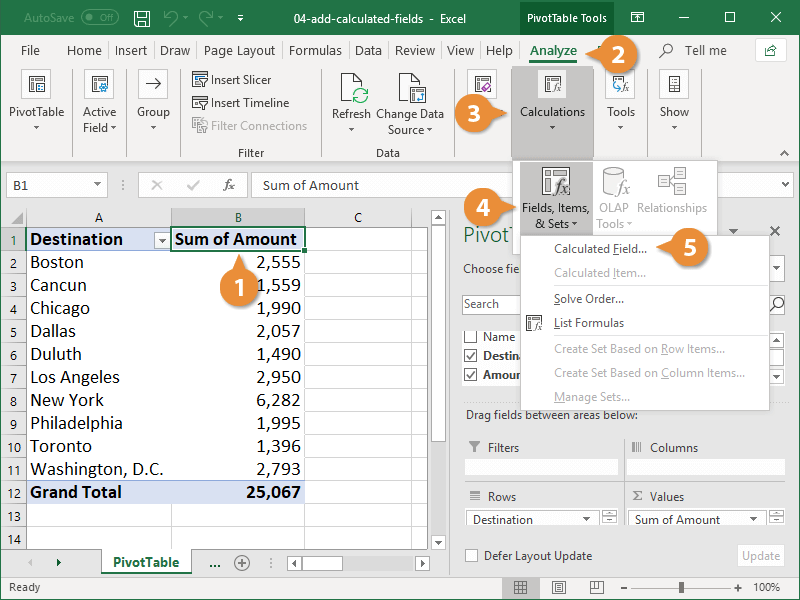
The following video provides an excellent, practical walkthrough of creating two calculated fields: one for 'Profit' and another for 'Profit Percentage'.
How to use a Pivot Table Calculated Field?
This video from Computer Tutoring demonstrates the process clearly with a business-focused example.
First, watch the setup where the instructor adds the necessary fields to the PivotTable and formats them (setup and formatting). Next, observe the creation of the first calculated field, 'Profit' (creating the Profit field). Notice how the formula ='Received'+'Expenses' is constructed using the existing field names. Finally, see how you can use a newly created calculated field in another calculation by creating a 'Profit Percentage' field (creating Profit Percentage).
A key thing to remember, as noted in the How to Create Excel Pivot Table Calculated Field Examples article, is that calculated field formulas always operate on the sum of the underlying data for any field you reference, regardless of how that field is summarized in the PivotTable (e.g., as a Count or Average).
3. Creating Calculated Items
Calculated items are used when you want to perform math on the items within a single category. The most common use is to group several items into a new, single item. For instance, if you have sales data for individual countries, you could create a calculated item to show total sales for a continent.
To create one, you select an item in the field you want to modify, then go to PivotTable Analyze > Fields, Items, & Sets > Calculated Item.
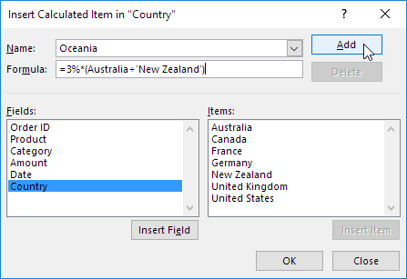
This video demonstrates how to combine several order statuses into a single 'Sold' category.
Excel Pivot Table Calculated Items and Calculated Fields
This video from Contextures Inc. provides a perfect example of creating a calculated item to group categories.
Watch the segment from creating a calculated item. Pay close attention to two critical details: How the formula is built by double-clicking the items (Backorder, Pending, Shipped). The final, crucial step of hiding the original items after the new 'Sold' item is created. If you don't do this, their values will be double-counted in the grand total.
While useful, calculated items have some restrictions. For example, once you add a calculated item to a field, you may not be able to use certain other PivotTable features on that field, like creating other custom groups. For this reason, calculated fields are generally preferred unless the calculation must be done across items.
4. Managing and Auditing PivotTable Formulas
As you build more complex reports, or when you inherit a workbook from someone else, you'll need a way to see all the custom formulas in a PivotTable. Excel provides a simple way to do this.
By selecting your PivotTable and navigating to PivotTable Analyze > Fields, Items, & Sets > List Formulas, Excel will instantly create a new worksheet that documents every calculated field and item in your PivotTable, showing their names and formulas.
Excel Pivot Table Calculated Items and Calculated Fields
The same Contextures video demonstrates this handy feature.
Watch the final part of the video explaining how to list all formulas. This is an invaluable technique for auditing and documenting your work.
To modify or delete a calculation, you simply return to the Calculated Field or Calculated Item dialog box, select the formula from the name dropdown, and click the Modify or Delete button.
5. Hands-On Practice
Let's apply what you've learned. Create a new Excel workbook and enter the following data into a worksheet.
| Date | Region | Product | Sales | Cost of Goods |
|---|---|---|---|---|
| 05-Jan-24 | North | Alpha | 500 | 350 |
| 05-Jan-24 | South | Beta | 400 | 280 |
| 06-Jan-24 | East | Alpha | 650 | 455 |
| 06-Jan-24 | West | Gamma | 300 | 210 |
| 07-Jan-24 | North | Beta | 800 | 560 |
| 07-Jan-24 | South | Gamma | 250 | 175 |
Step 1: Create a PivotTable
- Click inside your data range and go to Insert > PivotTable.
- Click OK to place the PivotTable on a new sheet.
- Set up the PivotTable as follows:
- Rows:
Region - Columns:
Product - Values:
Sum of Sales,Sum of Cost of Goods
- Rows:
Step 2: Create a Calculated Field
- Select a cell inside your PivotTable.
- Go to PivotTable Analyze > Fields, Items, & Sets > Calculated Field.
- In the
Namebox, type Profit. - In the
Formulabox, enter the formula:= Sales - 'Cost of Goods'(You can type it or double-click the field names from the list). - Click Add, then OK. A
Sum of Profitcolumn should now appear in your PivotTable.
Step 3: Create a Calculated Item
- Click on one of the region names (e.g., 'East') in the first column of your PivotTable.
- Go to PivotTable Analyze > Fields, Items, & Sets > Calculated Item.
- In the
Namebox, type Coastal. - In the
Formulabox, enter the formula:= East + West. - Click Add, then OK.
- You will now see a new 'Coastal' row. To avoid double-counting, right-click on the 'East' label, go to Filter > Hide Selected Items. Do the same for the 'West' label.
Your final PivotTable should now show data for North, South, and the new Coastal region, with columns for Sales, Cost of Goods, and the Profit you calculated.
Conclusion
You have now added a critical layer of analytical capability to your PivotTable skills. By using calculated fields and items, you can create new metrics and groupings on-the-fly, making your reports more insightful without cluttering your source data.
Key Takeaways:
- Calculated Fields create new columns and perform calculations between different fields (e.g.,
Price * Quantity). - Calculated Items create new rows and perform calculations between items in the same field (e.g.,
East + West). - Always be mindful of double-counting when using calculated items and hide the original items if necessary.
- Use the List Formulas command to quickly audit all custom calculations in a PivotTable.
In our next lesson, we will explore how to make your reports interactive. You'll learn how to add Slicers and Timelines, which are user-friendly filters that allow you or your clients to dynamically explore the data in your PivotTables with just a few clicks.