Introduction
In our previous lessons, we've mastered creating and customizing PivotTables from a single, flat data source. This is a powerful skill, but real-world data is rarely so tidy. More often, information is split across multiple tables—a list of sales transactions here, customer details there, and product information in yet another sheet.
In the past, you might have used functions like VLOOKUP or INDEX/MATCH to laboriously combine all this data into one giant table before making a PivotTable. This approach is inefficient, clutters your source data, and can make your files slow and difficult to maintain. Today, you'll learn a far more elegant and powerful solution: the Excel Data Model.
This lesson will show you how to create relationships between separate tables, effectively teaching Excel how they connect. Once these relationships are defined, you can build a single PivotTable that seamlessly pulls fields from all related tables, as if they were one. This is a fundamental technique for any serious data analysis and is a huge step toward building the sophisticated reports required in freelance projects.
1. The Concept of Relational Data
Before we dive into the "how," let's understand the "what." The Data Model works because it understands relational data structures. This typically involves two types of tables:
- Fact Tables: These contain records of transactions or events. For example, a table of every single sale made. This table can have many repeating values (e.g., the same customer ID appears every time that customer makes a purchase).
- Dimension Tables (or Lookup Tables): These contain unique lists of descriptive information, like a list of customers, products, or store locations. Each item (e.g., each customer ID) appears only once.
The two tables are linked by a common column, often called a key. This creates a one-to-many relationship: one customer in the dimension table can be linked to many sales in the fact table.
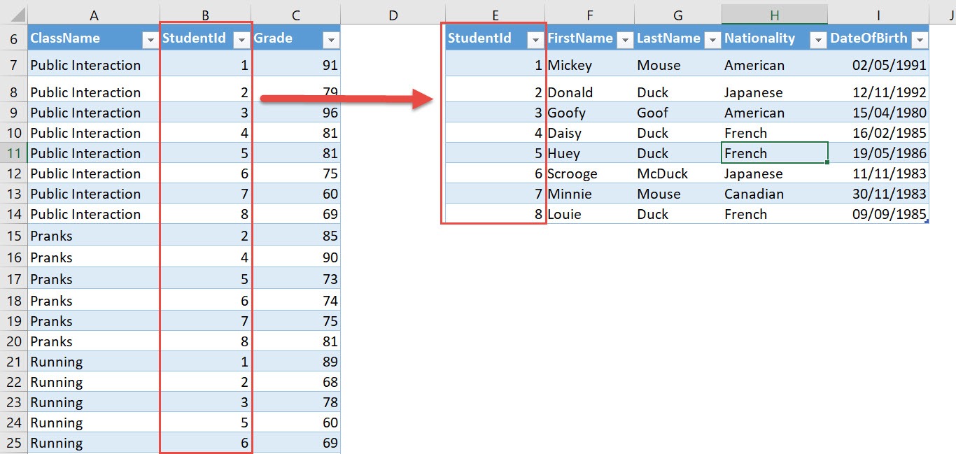
The most important rule for this to work is that the key column in the dimension (lookup) table must not contain any duplicate values. Let's see what happens when this rule is broken.
Excel Pivot Tables with Data Model & Multiple Tables are AWESOME!
The video "Excel Pivot Tables with Data Model" clearly explains the concept of one-to-many relationships and demonstrates the error that occurs when the rule of unique keys is violated.
Watch the segment from the explanation of relationships. Pay close attention to the distinction between the "facts table" (transactions) and the "related table" (products/customers). The presenter demonstrates what happens when a duplicate is added to the related table and the PivotTable is refreshed.
2. Building a PivotTable with the Data Model
There are a couple of ways to create a PivotTable using the Data Model. We'll explore two primary methods. First, a quick method where Excel prompts you to create relationships, and second, a more structured approach where you define the relationships upfront.
Method 1: Adding to the Data Model During PivotTable Creation
This is a fast way to get started. The key is a checkbox in the Create PivotTable dialog.
Excel Pivot Tables with Data Model & Multiple Tables are AWESOME!
The same video provides an excellent walkthrough of this first method.
First, watch how the raw data ranges are converted into proper Excel Tables with meaningful names (creating tables). This is a crucial prerequisite. Next, observe the process of creating a PivotTable. Notice the critical step of checking the box that says "Add this data to the Data Model" (adding to model). Finally, see what happens when you drag a field from a second table into the PivotTable. Excel recognizes the need for a relationship and prompts you to create one (creating a relationship).
This method is great for simple models, but for more complex reports, it's better to define your relationships proactively.
Method 2: Defining Relationships First
This more robust method involves telling Excel how your tables are related before you even create the PivotTable. This is the recommended approach for building clear and maintainable data models.
Let's look at another excellent resource that demonstrates this workflow.
Advanced Pivot Table Techniques: Combine Data from Multiple Sheets in Excel
Leila Gharani's video, "Advanced Pivot Table Techniques," provides a clear, business-oriented example of this structured approach.
Watch the introduction (the problem and data) to understand the scenario: a sales table (facts) needs to be linked to customer and article tables (dimensions). Next, see how relationships are created before the PivotTable using the Data > Relationships tool (building relationships). This is the core of this method. Finally, watch how to insert a PivotTable by selecting "Use this workbook's Data Model" and then easily pull fields from all three connected tables (creating the PivotTable).
For those who prefer a written guide, the following article walks through the exact same process with detailed screenshots.
How to Create a Pivot Table Based on Multiple Sheets and ...
This article from XelPlus provides a textual step-by-step guide for the structured approach.
Start by reading the sections on building relationships. This covers converting data to Tables, naming them, and using the Manage Relationships dialog. Then, review the section on populating the table, which reinforces how to create the PivotTable from the Data Model and add fields from different tables.
3. Managing and Visualizing Your Data Model
Once you've created relationships, you have a "Data Model" living inside your workbook. You can manage and visualize this model using the Power Pivot window.

To access this, go to the Data tab and click Manage Data Model. If this is your first time, Excel may ask you to enable the add-in.
The Power Pivot window has two main views:
- Data View: Looks like a spreadsheet, showing the data in each table.
- Diagram View: This is the most useful view. It displays your tables as boxes and the relationships as lines connecting them. You can see the "one" () and "many" () sides of each relationship.
This diagram is not just for viewing; you can also create, edit, or delete relationships by dragging and dropping fields between tables right here.
Advanced Pivot Table Techniques: Combine Data from Multiple Sheets in Excel
Leila Gharani's video also gives a concise tour of the Power Pivot window and a fantastic professional tip.
Watch the brief tour of the Power Pivot window, focusing on the Diagram View (Data Model views). Then, watch the section on hiding fields (hiding fields). This demonstrates how to hide the "key" columns (like CustomerID) from the PivotTable field list. This is excellent practice for creating clean, user-friendly reports for clients.
4. Hands-On Practice
It's time to build your own PivotTable from a Data Model. Create a new Excel workbook and follow these steps.
Step 1: Create Your Data Tables
Create three separate worksheets named Sales, Customers, and Products. Enter the following data on the corresponding sheets.
On the Sales sheet:
| OrderID | SaleDate | CustomerID | ProductID | Quantity |
|---|---|---|---|---|
| 1 | 01-Jan-2024 | C101 | P22 | 5 |
| 2 | 02-Jan-2024 | C102 | P33 | 2 |
| 3 | 02-Jan-2024 | C101 | P44 | 3 |
| 4 | 03-Jan-2024 | C103 | P22 | 10 |
| 5 | 04-Jan-2024 | C102 | P44 | 4 |
On the Customers sheet:
| CustomerID | CustomerName | Region |
|---|---|---|
| C101 | Global Corp | North |
| C102 | Innovate Inc. | South |
| C103 | Peak Systems | North |
On the Products sheet:
| ProductID | ProductName | Category |
|---|---|---|
| P22 | Alpha | Gadgets |
| P33 | Beta | Widgets |
| P44 | Gamma | Gadgets |
Step 2: Convert to Excel Tables
For each of the three data sets:
- Click anywhere inside the data.
- Press
Ctrl + T. - Ensure "My table has headers" is checked and click OK.
- Go to the Table Design tab and give each table a logical name:
tblSales,tblCustomers, andtblProducts.
Step 3: Create the Relationships
- Go to the Data tab -> Data Tools group -> Relationships.
- In the
Manage Relationshipsdialog, click New.... - Create the first relationship:
- Table:
tblSales - Column (Foreign):
CustomerID - Related Table:
tblCustomers - Related Column (Primary):
CustomerID - Click OK.
- Table:
- Click New... again to create the second relationship:
- Table:
tblSales - Column (Foreign):
ProductID - Related Table:
tblProducts - Related Column (Primary):
ProductID - Click OK.
- Table:
- You should now see both relationships listed. Click Close.
Step 4: Create the PivotTable
- Go to Insert -> PivotTable.
- In the
Create PivotTabledialog, select the option Use this workbook's Data Model. - Choose to place it on a new worksheet and click OK.
- In the PivotTable Fields list, you'll see all three tables.
- Build the report:
- From
tblProducts, drag Category to the Rows area. - From
tblCustomers, drag Region to the Columns area. - From
tblSales, drag Quantity to the Values area.
- From
You have now successfully created a PivotTable that summarizes data from three separate tables!
Conclusion
Congratulations, you have unlocked one of the most powerful features in Excel for data analysis. By moving away from manual VLOOKUP consolidations and embracing the Data Model, you can build reports that are faster, cleaner, and infinitely more scalable.
Key Takeaways:
- The Data Model allows you to create relationships between tables instead of merging them.
- Data is typically organized into Fact Tables (transactions) and Dimension Tables (lookups).
- Relationships are usually one-to-many, and the key column on the "one" side must have unique values.
- You can create relationships proactively via Data > Relationships and then build a PivotTable from the workbook's Data Model.
- The Power Pivot Diagram View is the best place to visualize and manage your data model.
In our next lesson, we will build upon this foundation. Now that you can construct sophisticated reports from multiple tables, we will explore how to add your own custom formulas directly into your PivotTables using Calculated Fields and Calculated Items.