Mini-Batch Gradient Descent Implementation

1. The Middle Ground: Understanding Mini-Batch Gradient Descent

Mini-batch gradient descent processes the data not one sample at a time, nor all at once, but in small groups called "mini-batches." For each mini-batch, we compute the average gradient and perform a parameter update. This approach has several key advantages:

• Efficiency: It's much faster than Batch GD because you don't have to process the entire dataset for a single update.
• Vectorization: Unlike single-sample SGD, it can take full advantage of optimized matrix operations in libraries like NumPy, as you're working with a small matrix (the mini-batch) instead of just one vector.
• Stability: By averaging gradients over a small batch (e.g., 32, 64, or 128 samples), the updates are less noisy than in SGD, leading to a more stable and reliable convergence.

Dr. Andrew Ng provides an excellent conceptual overview of mini-batch gradient descent in this video. It clearly explains how the data is partitioned and how the training process works.

As you saw in the video, we introduce two important terms:

• Batch Size: A hyperparameter that defines the number of samples in each mini-batch.
• Epoch: One complete cycle through all the training data. For a dataset with 1,000,000 samples and a batch size of 1000, one epoch would consist of 1,000 mini-batch updates.

2. Implementing Mini-Batch Gradient Descent from Scratch

Now, let's get to the implementation. The process involves two main steps: a function to create the mini-batches, and a main loop that iterates through them. We'll build upon the linear regression example from our previous lesson.

Step 1: Creating the Mini-Batches

The first new piece of logic we need is a function that takes our training data (X, y) and a batch_size, and returns a list of mini-batches.

A crucial step here is to shuffle the data at the beginning of each epoch. This ensures that the model sees a different combination of samples in each mini-batch during every epoch, which helps prevent the model from getting stuck in a poor local minimum and improves generalization. We must shuffle X and y together to maintain the correct input-output pairings.

The article "ML | Mini-Batch Gradient Descent with Python" from GeeksForGeeks provides a clear and effective function for this task.

Let's integrate this logic into our own implementation.

Step 2: The Full Implementation

Below is the complete code for mini-batch gradient descent. It combines the batch creation logic with the familiar training loop structure. Notice the nested loops: an outer loop for epochs and an inner loop for iterating through the mini-batches within each epoch.

import numpy as np
import matplotlib.pyplot as plt

# We'll use the same sample data as before
np.random.seed(42)
X = 2 * np.random.rand(100, 1)
y = 4 + 3 * X + np.random.randn(100, 1)

def create_mini_batches(X, y, batch_size):
    """
    Creates a list of random mini-batches from (X, y)
    """
    mini_batches = []
    # Horizontally stack X and y to shuffle them together
    data = np.hstack((X, y))
    np.random.shuffle(data)
    n_mini_batches = data.shape[0] // batch_size
    
    for i in range(n_mini_batches):
        mini_batch = data[i * batch_size:(i + 1) * batch_size, :]
        X_mini = mini_batch[:, :-1]
        y_mini = mini_batch[:, -1].reshape((-1, 1))
        mini_batches.append((X_mini, y_mini))
    
    # Handle the case of the last mini-batch, which may be smaller
    if data.shape[0] % batch_size != 0:
        mini_batch = data[n_mini_batches * batch_size:, :]
        X_mini = mini_batch[:, :-1]
        y_mini = mini_batch[:, -1].reshape((-1, 1))
        mini_batches.append((X_mini, y_mini))
        
    return mini_batches

def minibatch_gradient_descent(X, y, learning_rate, n_epochs, batch_size):
    """
    Implements mini-batch GD for a simple linear regression model.
    """
    # Add a column of ones to X for the bias term
    X_b = np.c_[np.ones((len(X), 1)), X]
    m, n_features = X_b.shape
    
    # Initialize weights randomly
    w = np.random.randn(n_features, 1)
    
    costs = []

    print(f"Starting Mini-Batch GD with batch_size={batch_size}...")
    for epoch in range(n_epochs):
        # 1. Create mini-batches for the current epoch
        mini_batches = create_mini_batches(X_b, y, batch_size)
        epoch_cost = 0
        
        # 2. Iterate through mini-batches
        for mini_batch in mini_batches:
            X_mini, y_mini = mini_batch
            
            # 3. Make prediction on the mini-batch
            y_pred = X_mini.dot(w)
            
            # 4. Calculate gradient for the mini-batch
            # This is the average gradient over the batch
            gradient = (2 / len(X_mini)) * X_mini.T.dot(y_pred - y_mini)
            
            # 5. Update weights
            w = w - learning_rate * gradient

            # Optional: track cost per mini-batch update for plotting
            cost = np.mean((y_pred - y_mini)**2)
            costs.append(cost)

    final_bias = w[0][0]
    final_weight = w[1][0]
    
    return final_weight, final_bias, costs

# --- Hyperparameters ---
LEARNING_RATE = 0.01
EPOCHS = 50
BATCH_SIZE = 16 # Configurable batch size

# --- Run the algorithm ---
w_final, b_final, mb_costs = minibatch_gradient_descent(X, y, LEARNING_RATE, EPOCHS, BATCH_SIZE)

print(f"\nDone! Final parameters -> Weight: {w_final:.4f}, Bias: {b_final:.4f}")

# Plotting the cost
plt.figure(figsize=(10, 6))
plt.plot(mb_costs)
plt.title(f'Mini-Batch GD Cost per Iteration (Batch Size = {BATCH_SIZE})')
plt.xlabel('Iteration (Mini-Batch update)')
plt.ylabel('Mean Squared Error')
plt.grid(True)
plt.show()

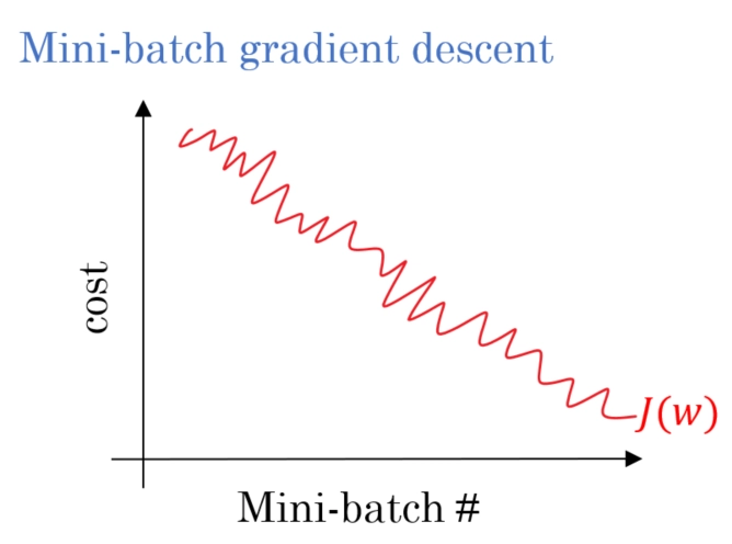
Run the code. The resulting plot shows the cost decreasing over iterations. Notice that the curve is "wavy" or noisy, but significantly less so than the SGD plot from our last lesson. This is the stabilization effect of averaging gradients over the mini-batch.

3. Comparing the Three Variants of Gradient Descent

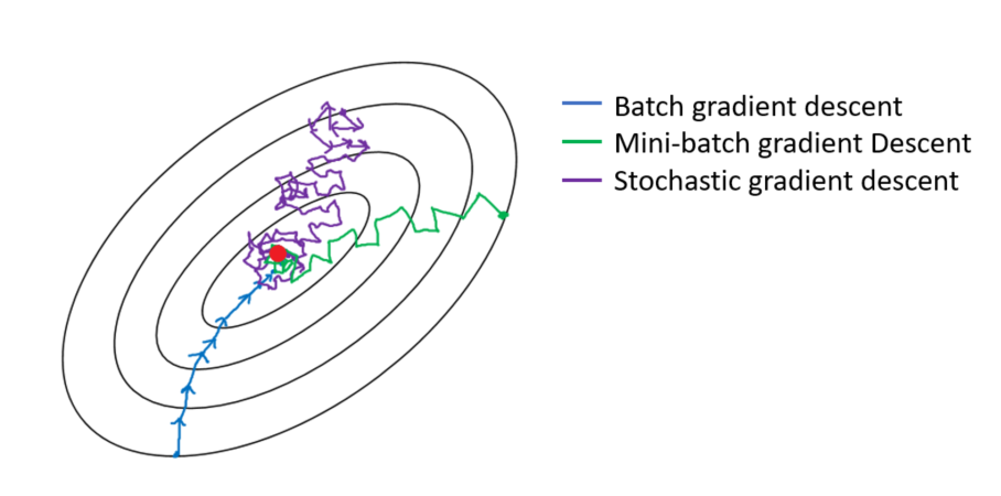
We have now implemented all three major variants of gradient descent. Each takes a different path to find the minimum of the loss function.

• Batch GD: Smooth, direct, but computationally expensive steps.
• Stochastic GD: Erratic, noisy, but computationally cheap steps.
• Mini-Batch GD: A balanced path—less noisy than SGD, but much more efficient than Batch GD.

This image provides a perfect visual summary of their different behaviors on a loss surface.

The batch_size is a critical hyperparameter that allows you to navigate the trade-off between these behaviors.

• If batch_size = 1, mini-batch GD becomes identical to SGD.
• If batch_size = m (the total number of samples), it becomes identical to Batch GD.
• In practice, batch_size is often a power of 2 (like 32, 64, 128, 256) to align with hardware memory architectures, but this is more of a convention than a strict rule.

Conclusion

Congratulations! You have now implemented the most widely-used optimization algorithm in machine learning. Mini-batch gradient descent provides a practical and efficient way to train models by balancing computational load with update stability.

Key Takeaways:

• Mini-Batch Gradient Descent updates parameters using the average gradient from a small subset (a mini-batch) of the training data.
• It combines the efficiency of vectorization with the rapid iteration of stochastic methods.
• Its convergence is less noisy than SGD but much faster than Batch GD.
• The batch_size is a key hyperparameter that controls the trade-off between update stability and computational speed.

Preview of the Next Lesson:
We've perfected our update frequency, but what about the update size? So far, we've used a fixed learning_rate. However, it's often beneficial to decrease the learning rate as training progresses, allowing for large steps at the beginning and finer adjustments near the minimum. In the next lesson, we will implement a simple learning rate scheduler to dynamically adjust the learning rate during training.