Learning Rate Scheduling for Optimization

1. The Intuition Behind a Decaying Learning Rate

Imagine you're trying to find the lowest point in a valley while blindfolded. At the start, you're high up on the slope, so you can confidently take large steps downhill. However, as you get closer to the bottom, the ground flattens out. If you keep taking large steps, you'll likely step right over the lowest point and end up on the other side. A smarter strategy would be to shorten your stride as the slope becomes less steep, allowing you to carefully find the absolute bottom.

This is exactly the intuition behind learning rate decay. We start with a relatively high learning rate ($\alpha$) to make quick progress, and then gradually decrease it over time (i.e., over epochs). This allows for fine-tuning as the optimizer gets closer to the minimum of the loss function.

To get a clear visual and conceptual understanding of this, watch the first part of the following video from DeepLearningAI.

2. Implementing Time-Based Decay from Scratch

There are many ways to schedule a learning rate decrease. We'll start with one of the most straightforward methods: time-based decay. The core idea is to make the learning rate a function of the epoch number. A common formula is:

${\alpha }_{\text{epoch}}=\frac{{\alpha }_0}{1+d\cdot \text{epoch}}$

Where:

• ${\alpha }_{\text{epoch}}$ is the learning rate for the current epoch.
• ${\alpha }_0$ is the initial learning rate (a hyperparameter).
• $d$ is the decay rate (another hyperparameter that controls how quickly $\alpha$ decreases).
• $\text{epoch}$ is the current epoch number (starting from 0 or 1).

Let's modify the minibatch_gradient_descent function from our last lesson to incorporate this scheduler. The changes are minimal: we'll add decay_rate as a parameter and update the learning rate at the start of each epoch loop.

Here is the updated code. Note the new line inside the for epoch in ... loop.

import numpy as np
import matplotlib.pyplot as plt

# We'll use the same sample data as before
np.random.seed(42)
X = 2 * np.random.rand(100, 1)
y = 4 + 3 * X + np.random.randn(100, 1)

def create_mini_batches(X, y, batch_size):
    mini_batches = []
    data = np.hstack((X, y))
    np.random.shuffle(data)
    n_mini_batches = data.shape[0] // batch_size
    
    for i in range(n_mini_batches):
        mini_batch = data[i * batch_size:(i + 1) * batch_size, :]
        X_mini = mini_batch[:, :-1]
        y_mini = mini_batch[:, -1].reshape((-1, 1))
        mini_batches.append((X_mini, y_mini))
    
    if data.shape[0] % batch_size != 0:
        mini_batch = data[n_mini_batches * batch_size:, :]
        X_mini = mini_batch[:, :-1]
        y_mini = mini_batch[:, -1].reshape((-1, 1))
        mini_batches.append((X_mini, y_mini))
        
    return mini_batches

# --- Updated function with learning rate scheduler ---
def minibatch_gd_with_scheduler(X, y, initial_lr, n_epochs, batch_size, decay_rate=0.1):
    """
    Implements mini-batch GD with a time-based decay learning rate scheduler.
    """
    X_b = np.c_[np.ones((len(X), 1)), X]
    m, n_features = X_b.shape
    w = np.random.randn(n_features, 1)
    
    costs = []
    learning_rates = [] # To track the LR over time

    print(f"Starting Mini-Batch GD with initial_lr={initial_lr} and decay_rate={decay_rate}...")
    for epoch in range(n_epochs):
        # --- THIS IS THE NEW PART ---
        # Update the learning rate for the current epoch
        lr = initial_lr / (1 + decay_rate * epoch)
        learning_rates.append(lr)
        
        mini_batches = create_mini_batches(X_b, y, batch_size)
        
        for mini_batch in mini_batches:
            X_mini, y_mini = mini_batch
            y_pred = X_mini.dot(w)
            gradient = (2 / len(X_mini)) * X_mini.T.dot(y_pred - y_mini)
            
            # Use the dynamically calculated learning rate for the update
            w = w - lr * gradient

            cost = np.mean((y_pred - y_mini)**2)
            costs.append(cost)

    final_bias = w[0][0]
    final_weight = w[1][0]
    
    return final_weight, final_bias, costs, learning_rates

# --- Hyperparameters ---
INITIAL_LEARNING_RATE = 0.1
EPOCHS = 50
BATCH_SIZE = 16
DECAY_RATE = 0.1 # New hyperparameter for the scheduler

# --- Run the algorithm ---
w_final, b_final, costs_sched, lrs = minibatch_gd_with_scheduler(
    X, y, INITIAL_LEARNING_RATE, EPOCHS, BATCH_SIZE, DECAY_RATE
)

print(f"\nDone! Final parameters -> Weight: {w_final:.4f}, Bias: {b_final:.4f}")

# --- Plotting the results ---
fig, (ax1, ax2) = plt.subplots(1, 2, figsize=(15, 6))

# Plot 1: Cost per iteration
ax1.plot(costs_sched)
ax1.set_title('Cost per Iteration with LR Scheduler')
ax1.set_xlabel('Iteration (Mini-Batch update)')
ax1.set_ylabel('Mean Squared Error')
ax1.grid(True)

# Plot 2: Learning Rate per Epoch
ax2.plot(range(EPOCHS), lrs)
ax2.set_title('Learning Rate Decay Over Epochs')
ax2.set_xlabel('Epoch')
ax2.set_ylabel('Learning Rate')
ax2.grid(True)

plt.show()

When you run this code, you'll see two plots. The first shows the cost decreasing, likely with less noise towards the end compared to a fixed learning rate. The second plot visually confirms that the learning rate is decreasing with each epoch, as intended.

3. Exploring Other Common Schedulers

Time-based decay is just one of many strategies. It's useful to be aware of a few others, as different schedulers can work better for different problems. The article below provides concise explanations, code, and visualizations for several popular schedulers.

Let's briefly summarize the key ideas from the article:

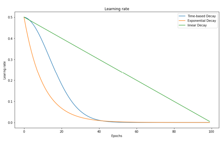
• Step Decay: The learning rate is reduced by a certain factor every N epochs. This creates a staircase-like decay pattern. For example, you might halve the learning rate every 10 epochs. This is very intuitive and easy to implement.
• Exponential Decay: The learning rate is multiplied by a factor less than 1 after every single epoch, resulting in a smooth, exponential curve. The formula is ${\alpha }_{\text{epoch}}={\alpha }_0\cdot e^{-k\cdot \text{epoch}}$.

This image provides a great side-by-side comparison of how different decay strategies reduce the learning rate over time.

4. Connection to Modern Frameworks

As you might expect, you rarely need to implement these schedulers from scratch in practice. Deep learning frameworks like PyTorch and TensorFlow have extensive, built-in libraries for learning rate scheduling.

For example, in PyTorch, you would typically:

1. Define your optimizer (e.g., torch.optim.SGD).
2. Define a scheduler and attach it to the optimizer (e.g., torch.optim.lr_scheduler.StepLR).
3. Inside your training loop, after you call optimizer.step(), you call scheduler.step().

The Patrick Loeber video PyTorch LR Scheduler gives a great tour of how this works in a real framework. While you don't need to watch it all now, it's good to know that the from-scratch logic you just implemented directly maps to these powerful, pre-built tools. For instance, the StepLR scheduler shown from 07:28 to 08:41 in the video implements the exact Step Decay logic we just discussed.

Conclusion

You've now added a powerful tool to your optimization arsenal! By implementing a learning rate scheduler, you've moved from a static optimization process to a dynamic one that can adapt over the course of training.

Key Takeaways:

• A learning rate scheduler dynamically adjusts the learning rate during training.
• The common strategy is to decay the learning rate, starting large for fast initial progress and decreasing for fine-tuning near the minimum.
• We implemented time-based decay from scratch by making the learning rate a function of the epoch number.
• Other common methods include Step Decay and Exponential Decay, each offering a different "cooldown" profile for the optimizer.

Preview of the Next Lesson:
This lesson concludes our module on the mechanics of optimization with gradient descent. We've built the engine; now it's time to build the car. In the next module, we will start our first "from scratch" model implementation: Linear Regression. Our first step will be to formally define its loss function—Mean Squared Error (MSE)—and derive its gradient. This will be the crucial mathematical step that allows us to apply our gradient descent optimizer to a real-world machine learning problem.