MSE Gradient for Linear Regression

1. The Linear Regression Model and its Error

At its heart, simple linear regression is about finding the best-fitting straight line through a set of data points. You might remember the equation of a line from school:

$y=mx+b$

In machine learning, we use slightly different notation, but the concept is identical. We have:

• Features ($x$): The input variable we use to make a prediction (e.g., square footage of a house).
• Target ($y$): The value we want to predict (e.g., price of a house).
• Parameters ($m,b$): The slope ($m$) and y-intercept ($b$) of the line. These are the values the model needs to learn from the data. We often call them weights and bias.

The model's prediction, which we'll call $\hat{y}$ ("y-hat"), is given by:

$\hat{y}=mx+b$

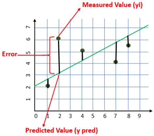
The "best" line is the one that minimizes the error between its predictions ($\hat{y}$) and the actual target values ($y$).

2. Quantifying Error with Mean Squared Error (MSE)

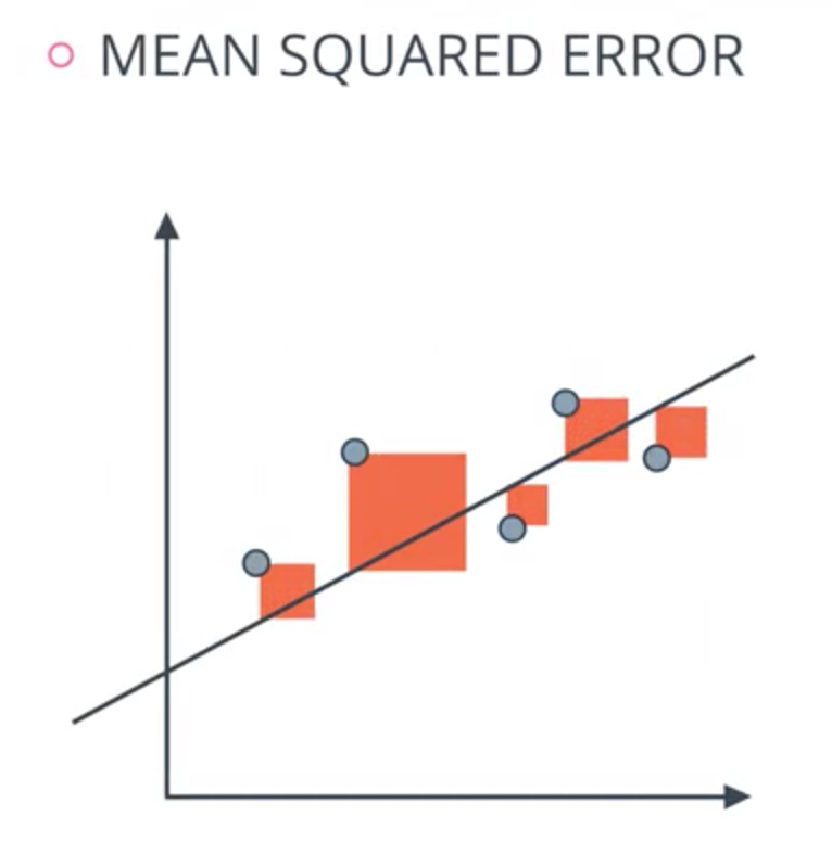
To find the best line, we need a single number that tells us how "bad" the current line is. This number is calculated by a loss function (or cost function). For linear regression, the most common loss function is the Mean Squared Error (MSE).

The MSE is calculated as follows:

1. For each data point, calculate the error: $y_i-{\hat{y}}_i$.
2. Square this error: $(y_i-{\hat{y}}_i{)}^2$. Squaring ensures all errors are positive and heavily penalizes large errors.
3. Average these squared errors across all $n$ data points.

This gives us the formula for MSE, which we'll call $J$:

$J(m,b)=\frac{1}{n}{\sum }_{i=1}^n(y_i-{\hat{y}}_i{)}^2=\frac{1}{n}{\sum }_{i=1}^n(y_i-(m{x}_i+b){)}^2$

Our goal is to find the values of $m$ and $b$ that result in the lowest possible $J$.

To get a clear walkthrough of these concepts, the following video provides an excellent introduction.

3. Deriving the Gradient of MSE

Now for the main task. To use gradient descent, we need the gradient of the loss function $J(m,b)$. The gradient is a vector containing the partial derivatives of the loss function with respect to each of its parameters ($m$ and $b$).

$\nabla J(m,b)=\left[\begin{array}{c}\frac{\partial J}{\partial m}\\ \\ \frac{\partial J}{\partial b}\end{array}\right]$

These derivatives tell us how a small change in $m$ or $b$ will affect the total error $J$. This is exactly the information gradient descent needs to know which "direction" to step in to reduce the error.

We'll find each partial derivative using the chain rule from calculus.

Partial Derivative with respect to the slope, $m$

Let's find $\frac{\partial J}{\partial m}$. We'll treat $b$ as a constant.

1. Start with the MSE formula:
   $J(m,b)=\frac{1}{n}{\sum }_{i=1}^n(y_i-m{x}_i-b{)}^2$

2. Apply the chain rule:

   • The derivative of the outer function $(...{)}^2$ is $2\cdot (...)$.
   • The derivative of the inner function $(y_i-m{x}_i-b)$ with respect to $m$ is $-x_i$.

3. Combine and simplify:

   $$\frac{\partial J}{\partial m}=\frac{1}{n}\sum _{i=1}^{n}2(y_i-m{x}_i-b)\cdot (-x_i)$$ $$\frac{\partial J}{\partial m}=-\frac{2}{n}\sum _{i=1}^n(y_i-(m{x}_i+b))\cdot x_i$$

   Since ${\hat{y}}_i=m{x}_i+b$, we can write this more cleanly as:

   $$\frac{\partial J}{\partial m}=-\frac{2}{n}\sum _{i=1}^n(y_i-{\hat{y}}_i)\cdot x_i$$

Partial Derivative with respect to the intercept, $b$

The process for $\frac{\partial J}{\partial b}$ is very similar. This time, we treat $m$ as a constant.

1. Start with the MSE formula again:
   $J(m,b)=\frac{1}{n}{\sum }_{i=1}^n(y_i-m{x}_i-b{)}^2$

2. Apply the chain rule:

   • The derivative of the outer function is the same: $2\cdot (...)$.
   • The derivative of the inner function $(y_i-m{x}_i-b)$ with respect to $b$ is $-1$.

3. Combine and simplify:

   $$\frac{\partial J}{\partial b}=\frac{1}{n}\sum _{i=1}^{n}2(y_i-m{x}_i-b)\cdot (-1)$$ $$\frac{\partial J}{\partial b}=-\frac{2}{n}\sum _{i=1}^n(y_i-(m{x}_i+b))$$

   And in terms of ${\hat{y}}_i$:

   $$\frac{\partial J}{\partial b}=-\frac{2}{n}\sum _{i=1}^n(y_i-{\hat{y}}_i)$$

The following video segment walks through this exact derivation step-by-step.

For a more formal, text-based explanation that also introduces the common vector notation used in machine learning literature, the following resource is excellent.

4. Calculating the Gradient in NumPy

With the math done, let's translate our final formulas into Python code. Given your background in NumPy, this should feel very natural. The summation $\sum$ and averaging $\frac{1}{n}$ can be handled efficiently with np.mean().

Let's set up a small example and calculate the gradient at a specific point.

import numpy as np

# Sample data
X = np.array([1, 2, 3, 4, 5])
y = np.array([2.1, 3.9, 6.2, 7.8, 10.1])

# Let's assume our model has some initial parameters
m = 1.5
b = 1.0

# 1. Calculate the predictions (y_hat)
y_pred = m * X + b
print(f"Predictions (y_hat): {y_pred}")

# 2. Calculate the errors (residuals)
errors = y - y_pred
print(f"Errors (y - y_hat): {errors}")

# 3. Calculate the partial derivatives using our derived formulas
# dJ/dm = -2/n * sum((y - y_hat) * x)
# which is equivalent to -2 * mean((y - y_hat) * x)
gradient_m = -2 * np.mean(errors * X)

# dJ/db = -2/n * sum(y - y_hat)
# which is equivalent to -2 * mean(y - y_hat)
gradient_b = -2 * np.mean(errors)

print("\n--- Gradient ---")
print(f"Partial derivative w.r.t. m (dJ/dm): {gradient_m:.4f}")
print(f"Partial derivative w.r.t. b (dJ/db): {gradient_b:.4f}")

The output values dJ/dm and dJ/db form our gradient vector $\nabla J$.

• gradient_m = -4.8400 tells us that if we increase m, the MSE will decrease (because the gradient is negative).
• gradient_b = -1.1600 tells us that if we increase b, the MSE will also decrease.

Gradient descent will use this information to update the parameters in the correct direction:

• m_new = m_old - learning_rate * gradient_m
• b_new = b_old - learning_rate * gradient_b

We will implement this update step in the next lesson.

Conclusion

Fantastic work! You've successfully connected the abstract concept of an optimizer to a concrete machine learning model. You now understand not just what the MSE loss function is, but also how to find its derivative—the engine of gradient-based learning.

Key Takeaways:

• Linear regression models learn the parameters (slope m and intercept b) of a line that best fits the data.
• The Mean Squared Error (MSE) is the standard loss function for regression, measuring the average squared distance between predictions and actual values.
• The gradient of the MSE is a vector of its partial derivatives with respect to each parameter ($\frac{\partial J}{\partial m}$ and $\frac{\partial J}{\partial b}$).
• We derived these partial derivatives using the chain rule, resulting in two clean formulas that can be implemented efficiently in NumPy.
• This gradient vector tells the optimizer the direction of steepest ascent, so our gradient descent algorithm will move in the opposite direction to minimize the error.

Preview of the Next Lesson:
We have all the components we need. In the next lesson, we will put everything together to implement a vectorized version of linear regression using gradient descent and NumPy. You'll combine the gradient calculation from today with the optimizer you built in the last module to train your very first model from scratch.