Vectorized Linear Regression with NumPy

1. From Scalar Math to Vectorized Operations

In the last lesson, we worked with a single feature $x$, using the familiar equation $\hat{y}=mx+b$. This is great for understanding the concepts, but real-world models often have dozens or even thousands of features. Iterating through each feature and each data point with Python for loops would be incredibly slow.

This is where vectorization comes in. By representing our data and parameters as matrices and vectors, we can leverage NumPy's highly optimized, low-level linear algebra operations to perform calculations on the entire dataset at once.

Let's update our notation for a multi-feature, multi-sample world:

• Features $X$: A matrix where each row is a data sample and each column is a feature. Its shape is (n_samples, n_features).
• Weights $W$: A vector containing the weight for each feature. Its shape is (n_features, 1).
• Bias $b$: A single scalar value, the same as the intercept from before.
• Targets $y$: A vector of the true values for each sample, with shape (n_samples, 1).
• Predictions $\hat{y}$: A vector of the model's predictions, with shape (n_samples, 1).

Our prediction equation $\hat{y}=m{x}_i+b$ for a single sample $i$ now becomes a powerful matrix equation for all samples at once:

$\hat{y}=X\cdot W+b$

Here, $X\cdot W$ is the dot product of the feature matrix and the weight vector. Let's look at the shapes to see how this works: (n_samples, n_features) dot (n_features, 1) results in a matrix of shape (n_samples, 1), which is exactly what we need for our predictions. NumPy handles this beautifully:

# Assuming X, W, and b are initialized
y_pred = np.dot(X, W) + b

2. The Vectorized Gradient

Just as we vectorized our prediction function, we can also vectorize our gradient calculations. Recall the partial derivatives we derived:

$\frac{\partial J}{\partial m}=-\frac{2}{n}{\sum }_{i=1}^n(y_i-{\hat{y}}_i)\cdot x_i\text{and}\frac{\partial J}{\partial b}=-\frac{2}{n}{\sum }_{i=1}^n(y_i-{\hat{y}}_i)$

In vectorized form, these become:

$\frac{\partial J}{\partial W}=\frac{2}{n}{X}^T(\hat{y}-y)$
$\frac{\partial J}{\partial b}=\frac{2}{n}\sum (\hat{y}-y)$

Let's break down the gradient with respect to the weights, $\frac{\partial J}{\partial W}$:

• $(\hat{y}-y)$ is the vector of errors, shape (n_samples, 1).
• $X^T$ is the transpose of the feature matrix, shape (n_features, n_samples).
• The dot product $X^T\cdot (\hat{y}-y)$ results in a shape of (n_features, 1), which is exactly the shape of our weight vector $W$. This gives us one gradient value for each weight, telling us how to update each one.

The Made With ML article provides a step-by-step breakdown of implementing these vectorized steps.

3. Implementing the LinearRegression Class

Now we'll assemble these components into a full-fledged LinearRegression class. This is a common and highly effective way to structure your machine learning code, keeping your model's logic self-contained. Our class will have three main methods:

1. __init__(self, learning_rate=0.01, n_iters=1000): The constructor to set hyperparameters like the learning rate and number of training iterations.
2. fit(self, X, y): The core training method that implements the gradient descent loop.
3. predict(self, X): The method to make predictions on new, unseen data using the learned weights.

The fit method is where the magic happens. It will loop for a specified number of iterations, and in each iteration, it will:

1. Compute the predictions $\hat{y}$.
2. Compute the gradients $\frac{\partial J}{\partial W}$ and $\frac{\partial J}{\partial b}$.
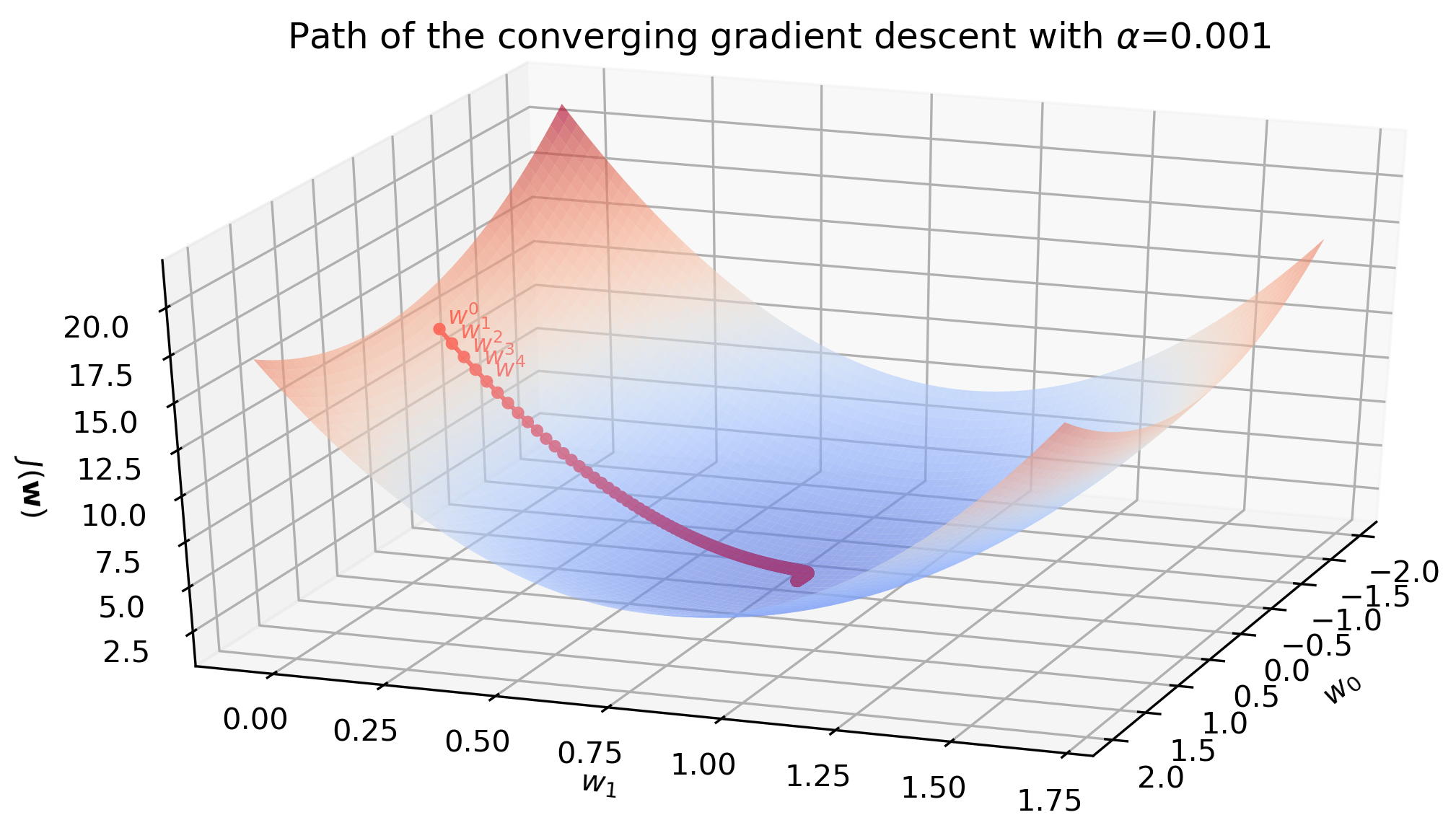
3. Update the parameters $W$ and $b$ using the gradient descent rule:
   $W:=W-\alpha \frac{\partial J}{\partial W}$
   $b:=b-\alpha \frac{\partial J}{\partial b}$

The following video provides a clear, from-scratch implementation of a very similar class structure. Watching it will help solidify your understanding of how the fit and predict methods work in practice.

4. Putting It All Together: Your First Model

Below is the complete, commented code for our vectorized LinearRegression class. It combines everything we've discussed: the vectorized prediction, the vectorized gradient calculation, and the iterative gradient descent update rule, all within a clean class structure.

import numpy as np

class LinearRegression:
    """
    A from-scratch implementation of Linear Regression using vectorized Gradient Descent.
    """
    def __init__(self, learning_rate=0.01, n_iters=1000):
        self.lr = learning_rate
        self.n_iters = n_iters
        self.weights = None
        self.bias = None

    def fit(self, X, y):
        """
        Train the linear regression model using gradient descent.
        X: Training data features, shape (n_samples, n_features)
        y: Training data targets, shape (n_samples,)
        """
        # 0. Initialize parameters
        n_samples, n_features = X.shape
        self.weights = np.zeros(n_features)
        self.bias = 0
        
        # Ensure y is the correct shape
        if y.ndim > 1:
            y = y.ravel()

        # 1. Gradient Descent
        for _ in range(self.n_iters):
            # Calculate predictions
            y_predicted = np.dot(X, self.weights) + self.bias
            
            # Calculate gradients based on our derived formulas
            # Note the factor of 2 from the derivative of the squared term
            dw = (2 / n_samples) * np.dot(X.T, (y_predicted - y))
            db = (2 / n_samples) * np.sum(y_predicted - y)
            
            # Update parameters
            self.weights -= self.lr * dw
            self.bias -= self.lr * db
            
    def predict(self, X):
        """
        Make predictions using the trained model.
        X: Data to make predictions on, shape (n_samples, n_features)
        """
        return np.dot(X, self.weights) + self.bias

5. Training and Evaluation

Let's see our model in action! We'll use scikit-learn to generate a synthetic regression dataset, split it, and then train and evaluate our from-scratch model.

# --- Imports for testing ---
from sklearn.model_selection import train_test_split
from sklearn.datasets import make_regression
import matplotlib.pyplot as plt

# --- A simple MSE function from Module 1 ---
def mean_squared_error(y_true, y_pred):
    return np.mean((y_true - y_pred)**2)

# 1. Generate synthetic data
X, y = make_regression(n_samples=100, n_features=1, noise=20, random_state=42)

# 2. Split data
X_train, X_test, y_train, y_test = train_test_split(X, y, test_size=0.2, random_state=1234)

# 3. Train our model
regressor = LinearRegression(learning_rate=0.01, n_iters=1000)
regressor.fit(X_train, y_train)

# 4. Make predictions
predictions = regressor.predict(X_test)

# 5. Evaluate the model
mse = mean_squared_error(y_test, predictions)
print(f"Mean Squared Error on test data: {mse:.2f}")

# 6. Visualize the results
y_pred_line = regressor.predict(X)
plt.figure(figsize=(8, 6))
plt.scatter(X_train, y_train, color='blue', label='Train data')
plt.scatter(X_test, y_test, color='green', label='Test data')
plt.plot(X, y_pred_line, color='red', linewidth=2, label='Prediction')
plt.title("Linear Regression from Scratch")
plt.xlabel("Feature")
plt.ylabel("Target")
plt.legend()
plt.show()

When you run this code, you'll see the calculated MSE and a plot showing how well your model's learned regression line fits the data.

Conclusion

Excellent work! You have now successfully built a complete, working linear regression model from the ground up using vectorized gradient descent. You've translated mathematical concepts into a reusable Python class and trained it on data.

Key Takeaways:

• Vectorization is key to writing efficient machine learning code, replacing slow Python loops with optimized NumPy operations.
• The prediction equation becomes $\hat{y}=XW+b$, and the gradient calculations for $W$ and $b$ have corresponding vectorized forms.
• A machine learning model can be cleanly encapsulated in a Python class with __init__, fit, and predict methods.
• The training loop is the heart of gradient descent, iteratively calculating predictions, computing gradients, and updating model parameters to minimize a loss function.

Preview of the Next Lesson:
Our model works, but can we make it train faster and more reliably? If you tried using a much larger learning rate in the code above, you might have seen the MSE explode. In the next lesson, we will explore why this happens and implement a crucial pre-processing step: feature normalization. You'll see how scaling your features can have a dramatic impact on the convergence speed of gradient descent.