SGD vs. Batch Gradient Descent: Convergence Comparison

1. The Need for Speed: Why Batch Gradient Descent Falters

The core issue with batch gradient descent is computational cost. As your dataset grows, the time it takes to compute the gradient for a single parameter update grows linearly. With modern datasets containing millions or even billions of samples, this becomes a critical bottleneck.

The following video from StatQuest gives an excellent and intuitive explanation of this problem, setting the stage perfectly for why an alternative like SGD is necessary.

2. The SGD Algorithm: One Sample at a Time

Stochastic Gradient Descent solves the speed problem with a simple but powerful change. Instead of aggregating gradients from all samples, it performs an update for every single sample.

The algorithm for one epoch looks like this:

1. Shuffle the training data: This is crucial to ensure the updates are truly random and not biased by any ordering in the data.
2. Iterate through each sample: For each (x_i, y_i) pair in the shuffled dataset:
   a. Calculate the loss and gradient for that single sample.
   b. Update the model parameters immediately using the update rule: parameters = parameters - learning_rate * gradient_i.

This means that for a dataset with 1,000,000 samples, SGD performs 1,000,000 small parameter updates per epoch, whereas batch GD would perform only one large, expensive update.

3. Implementing SGD from Scratch

Let's implement this. We'll adapt the structure from our last lesson, but instead of a generic objective_func, we'll frame it in the context of a simple linear regression model, just like in the codebasics video resource. Our goal will be to find the weights w and bias b for a model y_pred = w * x + b.

The code below implements the SGD loop. For now, we will use the analytical gradient formulas for the Mean Squared Error (MSE) loss of a single sample. Don't worry about their derivation; we'll cover that in detail in the next module. The key is to see how they are used inside the SGD loop.

import numpy as np
import matplotlib.pyplot as plt

# Let's create some sample data for linear regression
# X represents 'area' and y represents 'price'
np.random.seed(42)
X = 2 * np.random.rand(100, 1)
y = 4 + 3 * X + np.random.randn(100, 1)

def stochastic_gradient_descent(X, y, learning_rate, n_epochs):
    """
    Implements SGD for a simple linear regression model.
    
    Returns:
        tuple: A tuple containing the final weight, final bias, and a list of costs per epoch.
    """
    # Add a column of ones to X for the bias term (vectorized approach)
    X_b = np.c_[np.ones((len(X), 1)), X] 
    
    m, n_features = X_b.shape # m = number of samples
    
    # Initialize weights randomly
    w = np.random.randn(n_features, 1)
    
    costs = []

    print("Starting SGD...")
    for epoch in range(n_epochs):
        epoch_cost = 0
        
        # Shuffle the data at the start of each epoch
        shuffled_indices = np.random.permutation(m)
        X_shuffled = X_b[shuffled_indices]
        y_shuffled = y[shuffled_indices]

        for i in range(m):
            # 1. Pick a single random sample
            xi = X_shuffled[i:i+1]
            yi = y_shuffled[i:i+1]
            
            # 2. Make a prediction
            y_pred = xi.dot(w)
            
            # 3. Calculate the gradient for this single sample
            # This is the analytical gradient of MSE for one sample.
            # We'll derive this in the next module.
            gradient = 2 * xi.T.dot(y_pred - yi)
            
            # 4. Update the weights immediately
            w = w - learning_rate * gradient
            
            # Calculate cost for this sample and add to epoch cost
            cost = (y_pred - yi)**2
            epoch_cost += cost[0][0]

        # Store the average cost for the epoch
        costs.append(epoch_cost / m)
        if (epoch + 1) % 10 == 0:
            print(f"> Epoch {epoch+1}, Cost={costs[-1]:.4f}")
            
    # The first weight is the bias, the second is the weight for our feature
    final_bias = w[0][0]
    final_weight = w[1][0]
    
    return final_weight, final_bias, costs

# --- Hyperparameters ---
LEARNING_RATE = 0.01
EPOCHS = 50

# --- Run the algorithm ---
w_final, b_final, sgd_costs = stochastic_gradient_descent(X, y, LEARNING_RATE, EPOCHS)

print(f"\nDone! Final parameters -> Weight: {w_final:.4f}, Bias: {b_final:.4f}")

# Plotting the cost
plt.figure(figsize=(10, 6))
plt.plot(range(EPOCHS), sgd_costs)
plt.title('SGD Cost per Epoch')
plt.xlabel('Epoch')
plt.ylabel('Mean Squared Error')
plt.grid(True)
plt.show()

Notice the key differences from batch GD: the for i in range(m) loop inside the epoch loop, and the immediate update to w after processing each sample xi.

4. Comparing Convergence: Smooth vs. Noisy

Now for the crucial part of the learning outcome: comparing SGD to batch GD. Their convergence behaviors are strikingly different.

• Batch Gradient Descent moves directly towards the minimum. Since it averages the gradients of all data points, it takes a smooth, predictable path downhill.
• Stochastic Gradient Descent's path is erratic. The gradient of a single, random sample is a "noisy" but unbiased estimate of the true overall gradient. This causes the algorithm to zigzag and bounce around, but the general trend is towards the minimum.

This visual comparison is one of the most important concepts in optimization.

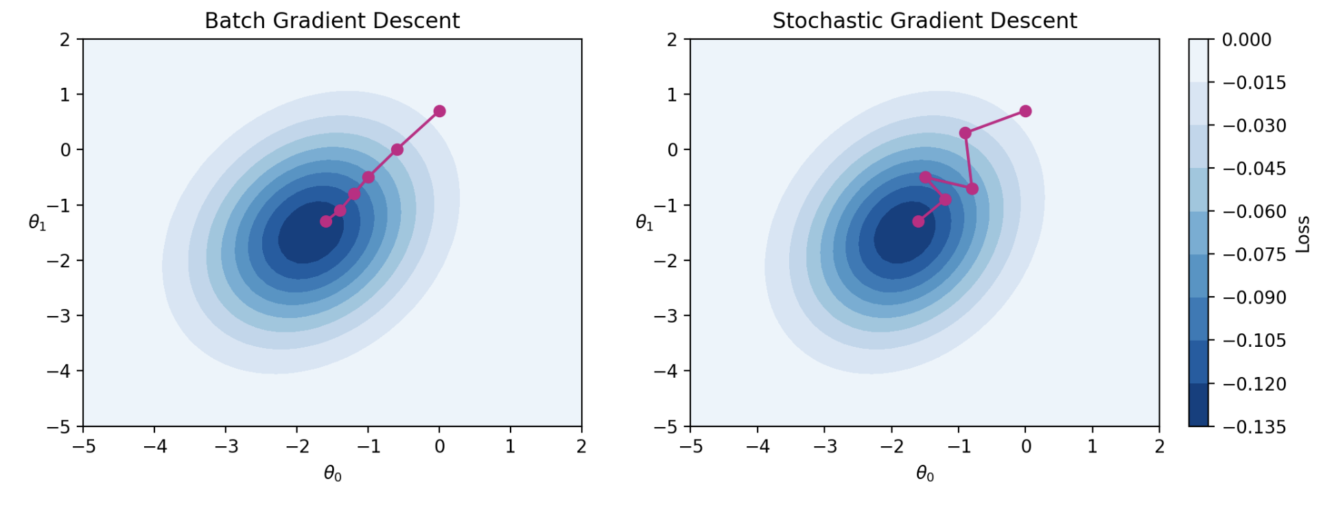
This noisy behavior is also reflected in the cost function plot. While the batch GD cost curve is a smooth, monotonically decreasing line, the SGD cost curve bounces up and down from one epoch to the next, even while trending downwards overall.

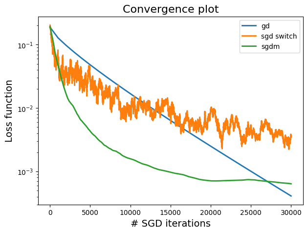
This "random walk" nature of SGD has an interesting side effect: its randomness can sometimes help it jump out of shallow local minima that might trap a smoother algorithm like batch GD.

Conclusion

You have now implemented SGD and seen firsthand how it trades smooth convergence for massive gains in computational speed. This trade-off is at the heart of modern machine learning, making it possible to train models on enormous datasets.

Key Takeaways:

• Stochastic Gradient Descent (SGD) updates model parameters using the gradient from a single random sample at a time.
• This makes SGD computationally far more efficient than batch GD for large datasets.
• The convergence path of SGD is noisy and erratic compared to the smooth path of batch GD.
• This noise can help SGD escape shallow local minima.
• The learning rate in SGD controls a trade-off between convergence speed and the stability of the descent.

Preview of the Next Lesson:
We've seen the two extremes: using all the data (batch) and using one sample (stochastic). Is there a middle ground? Yes! In the next lesson, we will implement Mini-Batch Gradient Descent, which combines the best of both worlds. It processes small batches of data at a time, offering a balance between the stability of batch GD and the efficiency of SGD, and is the most commonly used variant in practice.