Building a Training Loop

1. The Training Cycle

At its heart, training a neural network is a cyclical process. We make a guess, measure how wrong it is, and then use that error to make a slightly better guess. This cycle is repeated thousands of times.

This iterative process is often called the training loop. It has four main steps:

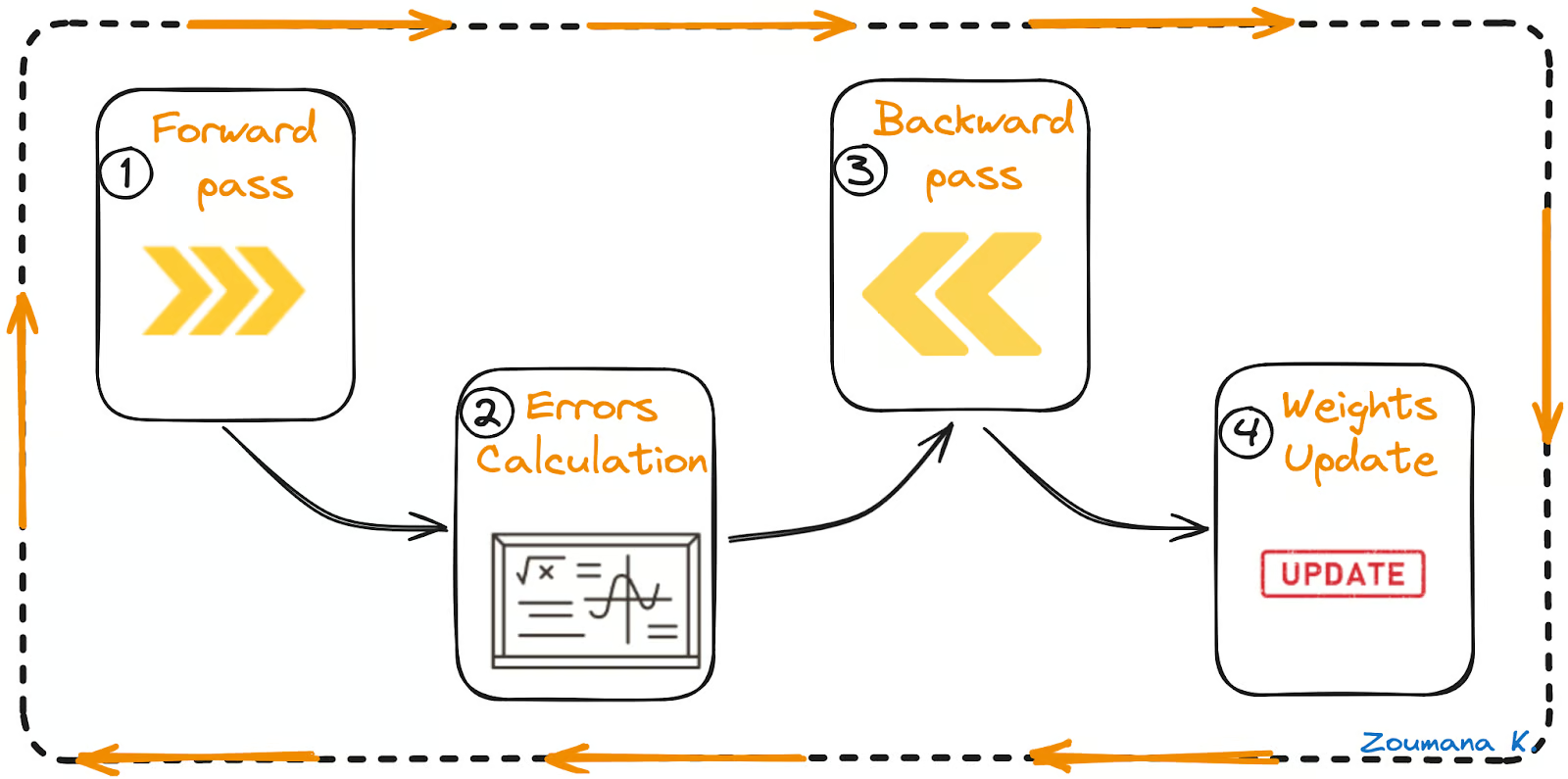
This entire process is an application of the gradient descent algorithm you've seen before. The "forward pass" and "loss calculation" define the value of our complex cost function $J(\theta )$, and the "backward pass" calculates the gradient $\nabla J(\theta )$. Finally, the "weight update" step takes a step down the gradient.

2. The Anatomy of the Training Loop

Let's translate that diagram into a concrete algorithm that you can implement. The main function, which we can call train_model or fit, will orchestrate these steps.

Here's the sequence of operations:

1. Initialization: Before the loop begins, initialize the network's parameters (weights W and biases b) for all layers. This happens only once.
2. Iteration: Start a loop that runs for a predefined number of iterations (or epochs).
3. Inside the Loop: For each iteration:
   a. Forward Propagation: Take the entire training dataset X and pass it through the network. This calculates the activations for each layer and produces the final predictions, Y_hat. You'll also need to store the intermediate values (Z and A from each layer) in a cache, as they are required for the backward pass.
   b. Cost Calculation: Compare the predictions Y_hat with the true labels Y using your cost function (e.g., cross-entropy) to get a single scalar value representing the total loss.
   c. Backward Propagation: Use the cache from the forward pass and the labels Y to compute the gradients of the cost with respect to every parameter (dW1, db1, dW2, db2, etc.).
   d. Parameter Update: Use the computed gradients and the learning rate (alpha) to update each parameter in the network. This is the classic gradient descent step: W = W - alpha * dW.
4. Completion: After the loop finishes, the parameters dictionary contains the learned weights and biases.

Let's watch a video that shows a developer implementing this exact logic in Python.

3. Implementing the Training Loop from Scratch

Now, let's formalize this into a code structure that you can build. You already have most of the necessary functions (initialize_parameters, forward_propagation, compute_cost, back_propagation). We just need to add the update_parameters function and the main train_model function to tie them all together.

The Parameter Update Function

Your back_propagation function returns a dictionary of gradients. The update function will take these gradients and the current parameters and apply the update rule.

Based on the video, your update_parameters function should look like this:

def update_parameters(parameters, gradients, learning_rate):
    """
    Updates parameters using the gradient descent update rule.

    Args:
        parameters (dict): Contains current parameters (W1, b1, ...).
        gradients (dict): Contains gradients from backprop (dW1, db1, ...).
        learning_rate (float): The learning rate alpha.

    Returns:
        dict: The updated parameters.
    """
    num_layers = len(parameters) // 2  # Number of layers in the network

    for l in range(1, num_layers + 1):
        parameters[f"W{l}"] = parameters[f"W{l}"] - learning_rate * gradients[f"dW{l}"]
        parameters[f"b{l}"] = parameters[f"b{l}"] - learning_rate * gradients[f"db{l}"]
        
    return parameters

The Main train_model Function

Now you can assemble everything into the main training function. This function will serve as the entry point for training your MLP.

def train_model(X, Y, layer_dims, num_iterations, learning_rate, print_cost=False):
    """
    Implements a L-layer neural network: [LINEAR->RELU]*(L-1)->LINEAR->SIGMOID/SOFTMAX.
    
    Args:
        X (np.array): Input data, of shape (input size, number of examples).
        Y (np.array): True "label" vector.
        layer_dims (list): List containing the input size and each layer size.
        num_iterations (int): Number of iterations of the optimization loop.
        learning_rate (float): Learning rate of the gradient descent update rule.
        print_cost (bool): If True, it prints the cost every 100 iterations.
    
    Returns:
        parameters (dict): Parameters learned by the model. They can then be used to predict.
        costs (list): A list of costs recorded during training.
    """
    costs = []
    
    # 1. Initialize parameters
    parameters = initialize_parameters(layer_dims)
    
    # 2. Start the training loop
    for i in range(num_iterations):
        
        # 3a. Forward propagation
        # For a classification network, AL is the final activation (sigmoid/softmax output)
        AL, cache = forward_propagation(X, parameters)
        
        # 3b. Compute cost
        cost = compute_cost(AL, Y)
        
        # 3c. Backward propagation
        gradients = back_propagation(AL, Y, cache)
        
        # 3d. Update parameters
        parameters = update_parameters(parameters, gradients, learning_rate)
        
        # Record and print the cost
        if print_cost and i % 100 == 0:
            print(f"Cost after iteration {i}: {cost}")
            costs.append(cost)
            
    return parameters, costs

4. Watching the Network Learn

You've built the engine. Now, how do you know if the car is moving? The most fundamental indicator of learning is a decreasing loss value.

The costs list that our train_model function returns is not just for printing; it's a vital diagnostic tool. By plotting the cost against the number of iterations, you can generate a loss curve. A healthy loss curve slopes downward, indicating that the model's predictions are getting closer to the true labels with each iteration.

Let's see a concrete example of this in action.

If you train your model and the loss stays flat, increases, or fluctuates wildly, it's a sign that something is wrong. Common culprits include:

• A bug in your backpropagation code (which you can verify with your gradient checker!).
• A learning rate that is too high (causing overshooting) or too low (causing negligible progress).
• Improper data normalization.

Conclusion

Congratulations! By assembling the training loop, you have created a fully functional, learning neural network from scratch. You now understand the complete end-to-end process, from feeding data forward to updating weights based on the calculated error.

Key Takeaways:

• The training loop is the central process that orchestrates learning in a neural network.
• It consists of four steps repeated iteratively: forward propagation, loss calculation, backward propagation, and parameter update.
• Parameters are initialized once before the loop begins, and are continuously refined within the loop.
• Monitoring the loss curve (cost vs. iterations) is the primary method for verifying that your model is learning correctly.

Preview of the Next Lesson:
Our current training loop uses the simplest form of gradient descent. While effective, it can sometimes be slow to converge. In the next lesson, you will implement the Momentum update rule, a popular technique to accelerate gradient descent and help it navigate complex loss landscapes more efficiently.