Accelerating SGD with Momentum

1. The Problem: The Winding Road of Gradient Descent

In the previous lesson, your update_parameters function took a simple step in the direction of the steepest descent: W = W - alpha * dW. This approach is greedy—it only considers the gradient at the current position. This can lead to two major problems:

1. Oscillations in Ravines: If the loss function forms a narrow, steep valley (a "ravine"), the gradient will point sharply down the walls. Standard GD will oscillate back and forth across the valley, making very slow progress along the valley floor toward the minimum.
2. Slowness on Plateaus: If the loss surface is very flat (a "plateau"), the gradients will be tiny, and GD will take very small, slow steps, drastically increasing training time.

Let's watch a short clip that illustrates this oscillation problem.

This animation of various optimizers navigating a loss surface vividly shows the zig-zagging path of basic SGD (the orange line) compared to more advanced methods.

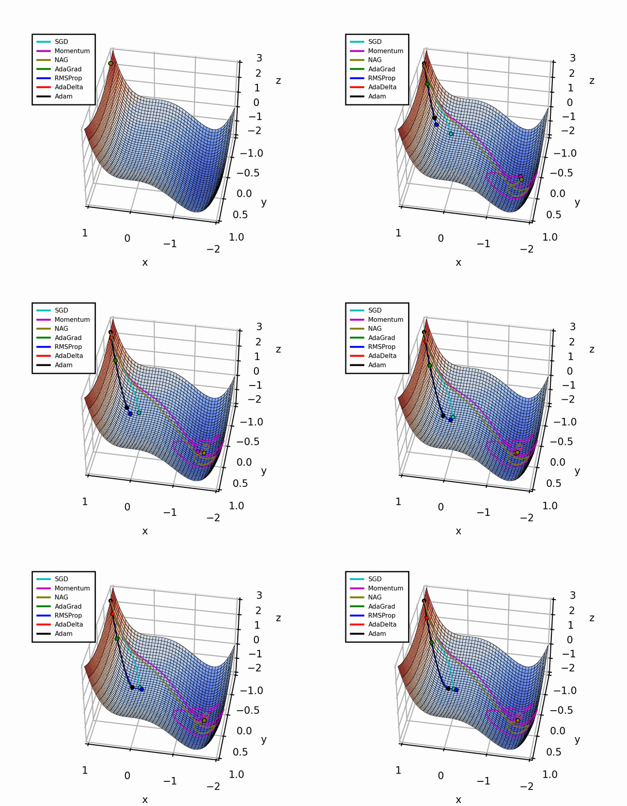
Our goal is to smooth out these oscillations and build "speed" in the correct direction.

2. The Intuition: A Ball Rolling Down a Hill

The core idea of Momentum is inspired by physics. Instead of a lightweight object that is pushed around by the gradient at every step, imagine a heavy ball rolling down the loss surface.

• The ball accumulates momentum, so it doesn't stop or change direction instantly.
• In a ravine, the oscillations from side to side will tend to cancel each other out, while the momentum carries it steadily down the valley floor.
• On a plateau, even with a small gradient (a gentle slope), its accumulated momentum will carry it forward.

This approach uses an exponentially weighted average of past gradients to inform the current update. In essence, it gives the update step a "memory" of which direction has been consistently good.

3. The Math Behind Momentum

To translate this physical intuition into an algorithm, we introduce a new variable called velocity (denoted by v), which will accumulate the weighted average of the gradients. At each step t, we perform two calculations:

1. Update the velocity: The new velocity is a combination of the old velocity and the current gradient.
2. Update the parameters: The parameters are updated using this new velocity instead of the raw gradient.

For a weight matrix W, the equations are:

Let's break this down:

• $v_{dW}^{(t)}$ is the velocity of the gradient of W at the current step t.
• $\beta$ is the momentum hyperparameter. It controls how much of the past velocity is retained. A common value is 0.9. If $\beta =0$, the equations collapse back to vanilla gradient descent.
• $d{W}^{(t)}$ is the gradient calculated at the current step t.
• $\alpha$ is the learning rate, as before.

The velocity $v_{dW}$ is an exponentially weighted average of the gradients. The term $(1-\beta )$ is a normalization factor that keeps the magnitude of the velocity in a similar range to the gradient itself. This specific formulation is popular because it makes the learning rate $\alpha$ less dependent on the value of $\beta$.

The following image provides a concise summary of the update rule and its implementation in pseudocode.

4. Implementing the Momentum Update Rule

Now, let's implement this. Since you have a strong background in Python and have already built the training scaffold, we can directly modify your existing structure. This will involve two changes:

1. Initializing a velocities dictionary to store the velocity terms for each parameter.
2. Creating a new update_parameters_with_momentum function that implements the equations above.

Step 1: Initialize the Velocities

Just like you initialized your parameters, you need a dictionary to hold the velocity terms (v_dW, v_db, etc.). These should all start at zero. You can create a helper function for this.

import numpy as np

def initialize_velocities(parameters):
    """
    Initializes the velocity as a dictionary with keys "v_dW1", "v_db1", ...,
    and values as numpy arrays of zeros of the same shape as the corresponding
    gradients/parameters.
    
    Args:
        parameters (dict): Contains the parameters "W1", "b1", etc.
    
    Returns:
        v (dict): Contains the initialized velocities.
    """
    num_layers = len(parameters) // 2
    v = {}
    
    for l in range(1, num_layers + 1):
        v[f"v_dW{l}"] = np.zeros_like(parameters[f"W{l}"])
        v[f"v_db{l}"] = np.zeros_like(parameters[f"b{l}"])
        
    return v

Step 2: Create the New Update Function

This function will now take velocities, beta, and learning_rate as inputs. It will update the velocities and then use them to update the parameters.

def update_parameters_with_momentum(parameters, gradients, velocities, beta, learning_rate):
    """
    Update parameters using Momentum.
    
    Args:
        parameters (dict): Contains current parameters.
        gradients (dict): Contains gradients from backprop.
        velocities (dict): Contains the current velocities.
        beta (float): The momentum hyperparameter.
        learning_rate (float): The learning rate.
    
    Returns:
        parameters (dict): The updated parameters.
        velocities (dict): The updated velocities.
    """
    num_layers = len(parameters) // 2
    
    for l in range(1, num_layers + 1):
        # Update velocities
        velocities[f"v_dW{l}"] = beta * velocities[f"v_dW{l}"] + (1 - beta) * gradients[f"dW{l}"]
        velocities[f"v_db{l}"] = beta * velocities[f"v_db{l}"] + (1 - beta) * gradients[f"db{l}"]
        
        # Update parameters
        parameters[f"W{l}"] = parameters[f"W{l}"] - learning_rate * velocities[f"v_dW{l}"]
        parameters[f"b{l}"] = parameters[f"b{l}"] - learning_rate * velocities[f"v_db{l}"]
        
    return parameters, velocities

Step 3: Integrate into Your Training Loop

Finally, modify your train_model function to use these new components.

1. Call initialize_velocities before the loop starts.
2. Inside the loop, call update_parameters_with_momentum instead of your old update function.
3. Make sure to pass the velocities dictionary into the function and capture the updated version it returns.

Your training loop would now look something like this:

# In your main training function...
# ...
# Hyperparameters
learning_rate = 0.01
beta = 0.9 # Momentum hyperparameter

# 1. Initialize parameters and velocities
parameters = initialize_parameters(layer_dims)
velocities = initialize_velocities(parameters)

# 2. Start the training loop
for i in range(num_iterations):
    # Forward prop, compute cost, backprop...
    AL, cache = forward_propagation(X, parameters)
    cost = compute_cost(AL, Y)
    gradients = back_propagation(AL, Y, cache)
    
    # Update parameters with momentum
    parameters, velocities = update_parameters_with_momentum(parameters, gradients, velocities, beta, learning_rate)
    
    # ... rest of the loop (print cost, etc.)

Conclusion

You have now implemented one of the most fundamental improvements to gradient descent. By incorporating a velocity term that tracks an exponentially weighted average of past gradients, you've enabled your optimizer to move faster and more smoothly toward the minimum of the loss function.

Key Takeaways:

• Vanilla SGD can be inefficient, causing oscillations in ravines and slow progress on plateaus.
• Momentum addresses this by adding a velocity term, which acts as an exponentially weighted average of past gradients.
• The hyperparameter $\beta$ controls the "friction" of the system, with a typical value of 0.9 providing a good balance of memory and responsiveness.
• Implementing Momentum requires initializing a velocities dictionary and modifying the parameter update step to first update the velocity, then update the parameters using that velocity.

Preview of the Next Lesson:
Momentum gives our optimizer a sense of direction and speed. But what if we could also adapt the learning rate for each parameter individually? In our next and final lesson of this module, you will implement the Adam optimizer from scratch, a powerful algorithm that combines the idea of momentum with adaptive learning rates to create one of the most effective and popular optimizers in deep learning today.