Implementing Adam from Scratch

1. The Two Pillars of Adam

Adam builds upon two key ideas, one of which you're already familiar with:

1. Momentum: Uses an exponentially weighted average of past gradients to accelerate in the right direction. This is an estimate of the first moment (the mean) of the gradients.
2. RMSprop: Adapts the learning rate for each parameter individually. It uses an exponentially weighted average of the squared gradients to scale the updates. This is an estimate of the second moment (the uncentered variance).

Let's watch a video that breaks down how Adam is derived from these two predecessors.

As the video explained, Adam combines these two concepts to get the best of both worlds. The result is an optimizer that not only moves faster but also intelligently adjusts its step size for every single parameter in your network.

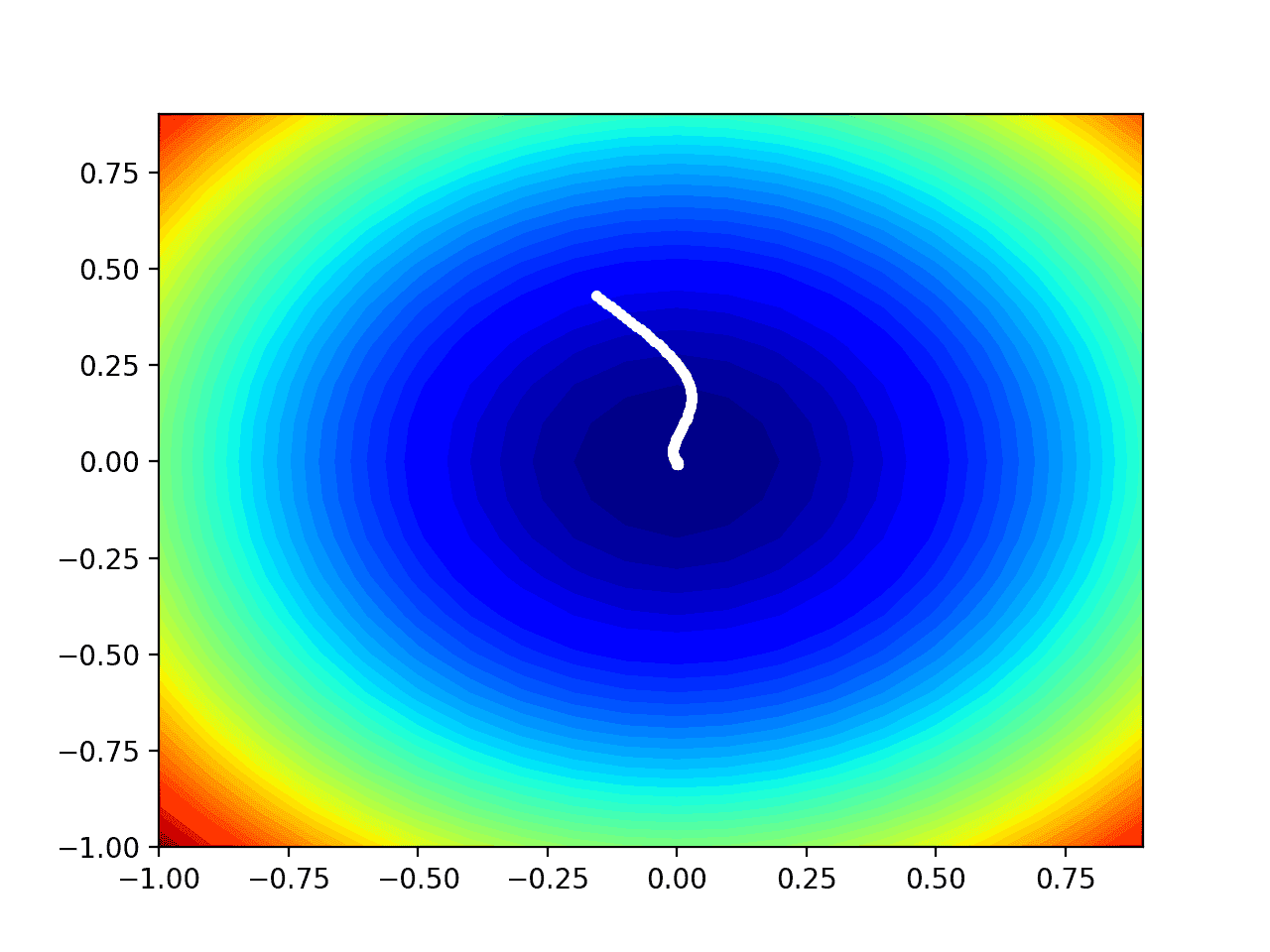
2. The Adam Algorithm: Math and Intuition

Let's assemble the complete Adam algorithm. At each timestep $t$, for each parameter (e.g., a weight matrix $W$), we perform the following steps:

1. Calculate Gradients: Compute $dW$ using backpropagation (you've already done this).

2. Update First Moment (Momentum):

   $$v_{dW}={\beta }_1{v}_{dW}+(1-{\beta }_1)dW$$

   This is exactly the momentum update you learned in the last lesson. $v_{dW}$ stores the exponentially weighted average of the gradients. ${\beta }_1$ is typically set to 0.9.

3. Update Second Moment (RMSprop):

   $$s_{dW}={\beta }_2{s}_{dW}+(1-{\beta }_2)d{W}^2$$

   This is the new part. $s_{dW}$ stores the exponentially weighted average of the squared gradients. $d{W}^2$ means element-wise squaring. ${\beta }_2$ is typically set to 0.999.

4. Apply Bias Correction: Since $v_{dW}$ and $s_{dW}$ are initialized to zero, they are biased towards zero during the first few iterations. To counteract this, we compute corrected values:

   $${\hat{v}}_{dW}=\frac{v_{dW}}{1-{\beta }_1^t}$$ $${\hat{s}}_{dW}=\frac{s_{dW}}{1-{\beta }_2^t}$$

   Here, $t$ is the current iteration number. As $t$ increases, the denominators approach 1, and the correction effect fades away.

5. Update Parameters: Finally, we update the weights using the bias-corrected moment estimates.

   $$W=W-\alpha \frac{{\hat{v}}_{dW}}{\sqrt{{\hat{s}}_{dW}}+ϵ}$$
   • $\alpha$ is the learning rate.
   • We divide the momentum term ${\hat{v}}_{dW}$ by the square root of the squared gradient term $\sqrt{{\hat{s}}_{dW}}$. This is the adaptive learning rate part. If past gradients for a parameter have been large (large ${\hat{s}}_{dW}$), the update step is made smaller. If they've been small, the update is larger.
   • $ϵ$ is a very small number (e.g., $10^{-8}$) to prevent division by zero.

For a clear walkthrough of these steps and the corresponding code, the following article is an excellent guide.

3. Implementing Adam From Scratch

Now, let's get to the code. Your experience with Python, NumPy, and your existing training framework will make this straightforward. We will create two new functions, initialize_adam and update_parameters_with_adam, which are direct extensions of the momentum functions from our last lesson.

Step 1: Initialize Adam Parameters

First, we need a function to initialize the moment estimates, v and s, for all our model's parameters. They should all start as zero arrays with the same dimensions as the parameters they correspond to.

import numpy as np

def initialize_adam(parameters):
    """
    Initializes v and s as dictionaries with keys ("v_dW1", "v_db1", ...) and
    ("s_dW1", "s_db1", ...), and values as numpy arrays of zeros of the same 
    shape as the corresponding gradients/parameters.
    
    Args:
        parameters (dict): Contains the parameters "W1", "b1", etc.
    
    Returns:
        v (dict): Contains the exponentially weighted average of the gradient.
        s (dict): Contains the exponentially weighted average of the squared gradient.
    """
    num_layers = len(parameters) // 2
    v = {}
    s = {}
    
    for l in range(1, num_layers + 1):
        v[f"v_dW{l}"] = np.zeros_like(parameters[f"W{l}"])
        v[f"v_db{l}"] = np.zeros_like(parameters[f"b{l}"])
        s[f"s_dW{l}"] = np.zeros_like(parameters[f"W{l}"])
        s[f"s_db{l}"] = np.zeros_like(parameters[f"b{l}"])
        
    return v, s

This looks very similar to initialize_velocities, but now it creates two dictionaries.

Step 2: Implement the Adam Update Rule

This is the main function. It will take the parameters, gradients, the v and s dictionaries, the current timestep t, and the hyperparameters as input. It then implements the 5-step process we just discussed.

The following video shows a live coding session that implements this logic.

Now, let's write our own version that fits neatly into your existing multi-layer network structure.

def update_parameters_with_adam(parameters, gradients, v, s, t, learning_rate=0.01,
                                beta1=0.9, beta2=0.999, epsilon=1e-8):
    """
    Update parameters using Adam.
    
    Args:
        parameters (dict): Contains current parameters.
        gradients (dict): Contains gradients from backprop.
        v (dict): Adam's first moment estimates.
        s (dict): Adam's second moment estimates.
        t (int): The current iteration number (for bias correction).
        learning_rate (float): The learning rate.
        beta1 (float): Exponential decay hyperparameter for the first moment.
        beta2 (float): Exponential decay hyperparameter for the second moment.
        epsilon (float): Hyperparameter to prevent division by zero.
    
    Returns:
        parameters (dict): Updated parameters.
        v (dict): Updated first moment estimates.
        s (dict): Updated second moment estimates.
    """
    num_layers = len(parameters) // 2
    v_corrected = {}
    s_corrected = {}
    
    for l in range(1, num_layers + 1):
        # 1. Update first moment estimates (v)
        v[f"v_dW{l}"] = beta1 * v[f"v_dW{l}"] + (1 - beta1) * gradients[f"dW{l}"]
        v[f"v_db{l}"] = beta1 * v[f"v_db{l}"] + (1 - beta1) * gradients[f"db{l}"]
        
        # 2. Compute bias-corrected first moment estimates
        v_corrected[f"v_dW{l}"] = v[f"v_dW{l}"] / (1 - beta1**t)
        v_corrected[f"v_db{l}"] = v[f"v_db{l}"] / (1 - beta1**t)
        
        # 3. Update second moment estimates (s)
        s[f"s_dW{l}"] = beta2 * s[f"s_dW{l}"] + (1 - beta2) * (gradients[f"dW{l}"]**2)
        s[f"s_db{l}"] = beta2 * s[f"s_db{l}"] + (1 - beta2) * (gradients[f"db{l}"]**2)
        
        # 4. Compute bias-corrected second moment estimates
        s_corrected[f"s_dW{l}"] = s[f"s_dW{l}"] / (1 - beta2**t)
        s_corrected[f"s_db{l}"] = s[f"s_db{l}"] / (1 - beta2**t)
        
        # 5. Update parameters
        parameters[f"W{l}"] -= learning_rate * (v_corrected[f"v_dW{l}"] / (np.sqrt(s_corrected[f"s_dW{l}"]) + epsilon))
        parameters[f"b{l}"] -= learning_rate * (v_corrected[f"v_db{l}"] / (np.sqrt(s_corrected[f"s_db{l}"]) + epsilon))
        
    return parameters, v, s

Step 3: Integrate into Your Training Loop

The final step is to incorporate these functions into your main training loop.

1. Before the loop, call initialize_adam to create the v and s dictionaries.
2. Initialize a timestep counter, t = 0.
3. Inside the loop, after calculating gradients, increment t and call update_parameters_with_adam.

Your training loop's core logic will now look like this:

# In your main training function...
# ...
# Hyperparameters
learning_rate = 0.0075
beta1 = 0.9
beta2 = 0.999
epsilon = 1e-8

# 1. Initialize parameters
parameters = initialize_parameters(layer_dims)

# 2. Initialize Adam variables
v, s = initialize_adam(parameters)
t = 0 # Initialize timestep counter

# 3. Start the training loop
for i in range(num_iterations):
    # Forward prop, compute cost, backprop...
    AL, cache = forward_propagation(X, parameters)
    cost = compute_cost(AL, Y)
    gradients = back_propagation(AL, Y, cache)
    
    # Increment timestep and update parameters with Adam
    t = t + 1
    parameters, v, s = update_parameters_with_adam(parameters, gradients, v, s, t, learning_rate, beta1, beta2, epsilon)
    
    # ... rest of the loop (print cost, etc.)

Conclusion

Congratulations! You have now implemented the Adam optimizer from scratch. This is a significant milestone, as Adam is a cornerstone of modern deep learning. You've successfully combined two powerful concepts—momentum and adaptive per-parameter learning rates—into a single, elegant algorithm.

Key Takeaways:

• Adam (Adaptive Moment Estimation) combines the benefits of Momentum (using past gradients to accelerate) and RMSprop (using past squared gradients to adapt learning rates).
• It maintains two moving averages: the first moment ($v$) for the mean of gradients and the second moment ($s$) for the uncentered variance of gradients.
• Bias correction is crucial in the early stages of training to counteract the zero-initialization of $v$ and $s$.
• The final update rule uses the corrected first moment as the numerator (like momentum) and the square root of the corrected second moment as the denominator (to scale the learning rate).

Preview of the Next Lesson:
You have now built a powerful neural network and mastered several optimization techniques. In our next module, we'll begin the capstone project. You'll first learn to implement early stopping to prevent overfitting automatically. Then, you will structure your code into a reusable pipeline to systematically train and evaluate every single algorithm you've built throughout this course on a benchmark dataset, creating a comprehensive report of their performance.