Gradient Checking for Backpropagation

1. The Problem: Silent Bugs in Backpropagation

As you've seen in your own projects, some bugs are obvious—they throw errors and crash your program. Other, more "nefarious" bugs, simply lead to incorrect results. A bug in backpropagation is often of the second kind. Your network might seem to train, with the loss decreasing slightly or fluctuating, but it never achieves good performance.

To understand why this is a common issue and why we need a solution, let's look at a video that frames the problem perfectly.

Gradient checking solves this by comparing the gradients calculated by backpropagation (the "analytical" gradients) with a numerical approximation of the gradients. If they match, our backprop code is correct.

2. The Solution: Numerical Gradient Approximation

How can we approximate a gradient without calculus? We can go back to the fundamental definition of a derivative. A derivative is simply the slope of a function at a point. We can approximate this slope by taking a very small step, ε (epsilon), and measuring the change in the function's output.

A simple way to do this is the one-sided formula: $\frac{f(x+ϵ)-f(x)}{ϵ}$. However, a more accurate and robust approximation uses a two-sided difference:

This formula calculates the slope of the line connecting the points on the function at $x-ϵ$ and $x+ϵ$, which is a much better approximation of the tangent at $x$, especially for curved functions.

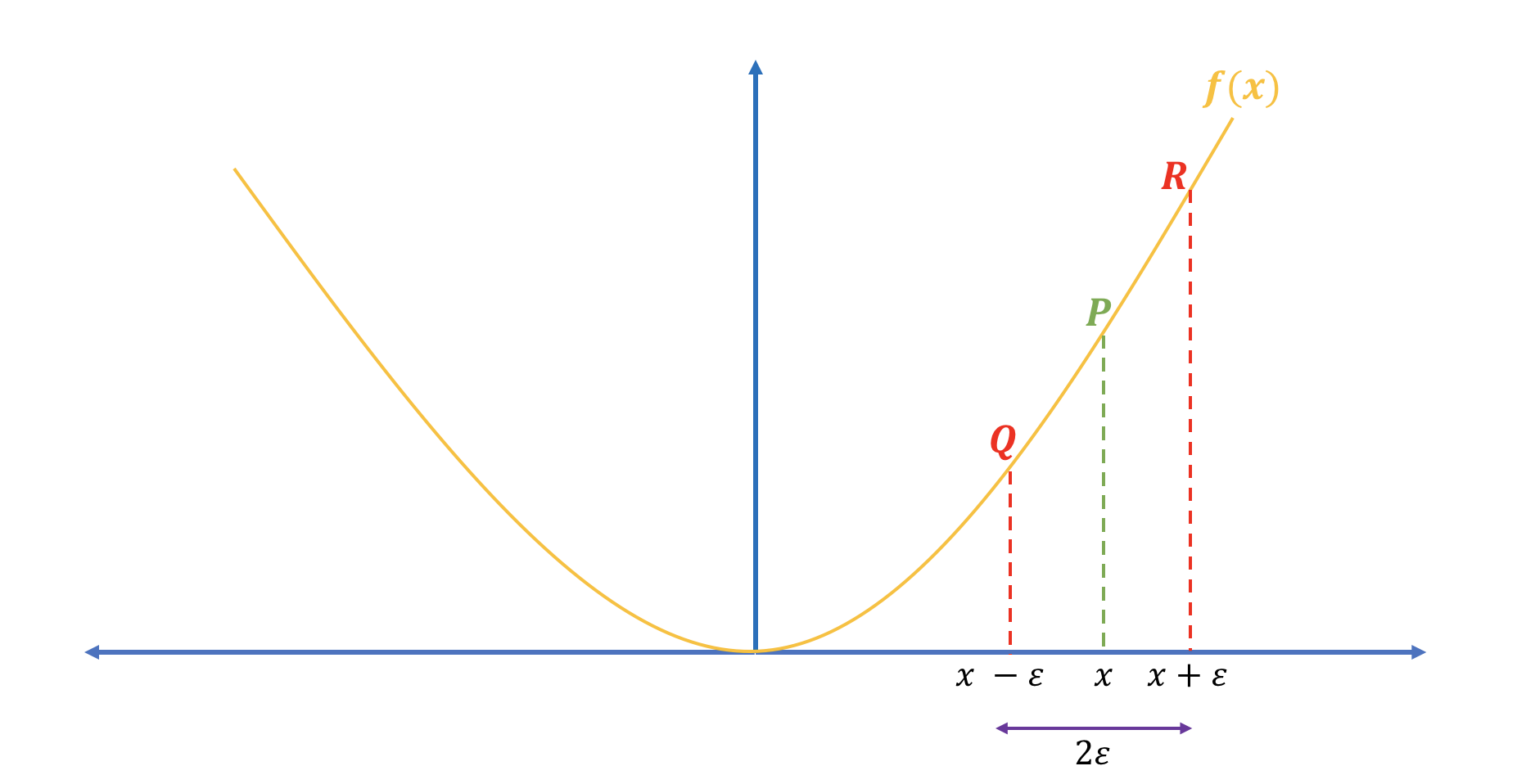
Our neural network's cost function, $J$, is just a very complex function of all its parameters (all the W's and b's). We can apply this exact principle to check the gradient for each and every parameter.

3. The Gradient Checking Algorithm

The overall strategy is to treat all the network's parameters as one giant vector. Let's call this vector θ. Our cost function is $J(\theta )$. Our backpropagation algorithm gives us dθ, the analytical gradient of $J$ with respect to θ.

To check this, we will compute a numerical gradient, dθ_approx, one element at a time:

1. For each parameter θ_i in our network:
   a. Calculate the cost when we slightly increase that single parameter: $J({\theta }_1,{\theta }_2,...,{\theta }_i+ϵ,...)$. Let's call this cost_plus.
   b. Calculate the cost when we slightly decrease it: $J({\theta }_1,{\theta }_2,...,{\theta }_i-ϵ,...)$. Let's call this cost_minus.
   c. The numerical gradient for this specific parameter is: dθ_approx[i] = (cost_plus - cost_minus) / (2 * ε).
2. Compare: After looping through all parameters, we will have two full gradient vectors: dθ (from backprop) and dθ_approx (from our numerical process). We then compute a measure of difference between them to see if they are close enough.

This process is computationally very expensive because it requires two forward passes through the entire network for every single parameter. This is why it's only used as a debugging tool, not during actual training.

Let's watch a detailed explanation of this process.

4. Implementing Gradient Checking from Scratch

Now for the part you prefer: implementing this in code. While the vectorized approach of unrolling parameters into a single theta vector is elegant, a more direct (and perhaps easier to debug) method uses nested loops to iterate through each parameter in its original matrix/vector shape.

Let's study a clear, from-scratch implementation that does exactly this.

Let's break down the logic of that code, which you will integrate into your own MLP project.

Here's the pseudocode for a gradient_check function:

def gradient_check(parameters, gradients, X, Y, epsilon=1e-7):
    """
    Checks if the backpropagation-computed gradients are correct.

    Args:
        parameters (dict): A dictionary of the network's parameters (e.g., {"W1": W1, "b1": b1, ...})
        gradients (dict): A dictionary of the backprop gradients (e.g., {"dW1": dW1, "db1": db1, ...})
        X (np.array): Input data.
        Y (np.array): True labels.
        epsilon (float): A very small number for perturbation.

    Returns:
        float: The relative difference between numerical and analytical gradients.
    """
    
    # Unroll parameters and gradients into vectors for easier comparison later
    params_vector = unroll(parameters)
    grad_vector = unroll(gradients)
    num_parameters = params_vector.shape[0]
    grad_approx_vector = np.zeros((num_parameters, 1))

    # Iterate through each parameter
    for i in range(num_parameters):
        # --- Calculate grad_approx[i] ---
        
        # 1. Perturb the i-th parameter by +epsilon
        params_plus = np.copy(params_vector)
        params_plus[i][0] += epsilon
        params_plus_dict = roll_up(params_plus, network_architecture) # Convert back to dict
        
        # 2. Run forward prop and get cost
        # Note: Your forward_prop function needs to accept the parameter dictionary
        cost_plus = calculate_cost(forward_prop(X, params_plus_dict), Y)

        # 3. Perturb the i-th parameter by -epsilon
        params_minus = np.copy(params_vector)
        params_minus[i][0] -= epsilon
        params_minus_dict = roll_up(params_minus, network_architecture)
        
        # 4. Run forward prop and get cost
        cost_minus = calculate_cost(forward_prop(X, params_minus_dict), Y)

        # 5. Compute the numerical gradient for this parameter
        grad_approx_vector[i] = (cost_plus - cost_minus) / (2 * epsilon)

    # --- Compare grad_approx_vector with grad_vector ---
    numerator = np.linalg.norm(grad_vector - grad_approx_vector)
    denominator = np.linalg.norm(grad_vector) + np.linalg.norm(grad_approx_vector)
    difference = numerator / denominator
    
    return difference

# You would need to implement helper functions 'unroll' and 'roll_up'
# to convert between the dictionary of parameters and the single vector.

5. Interpreting the Results

After all that computation, you get a single number: the difference. How do you interpret it? As Andrew Ng explained, here are some good rules of thumb:

• Difference < 10⁻⁷: Great! Your backpropagation implementation is very likely correct.
• Difference ≈ 10⁻⁵: This is a grey area. It might be okay, but you should double-check your code. This can sometimes happen due to using float32 precision instead of float64.
• Difference > 10⁻³: You almost certainly have a bug in your backpropagation code.

If you find a large difference, the real debugging begins. You can print the numerical and analytical gradients for each parameter to find the exact weight or bias where the calculation first goes wrong. This often points directly to the bug in your backprop formulas for that specific layer.

Conclusion

You now have a powerful tool for ensuring your neural network's learning mechanism is bug-free. Implementing gradient checking is a rite of passage for anyone building neural networks from scratch. It forces a deep understanding of the relationship between the forward pass (cost) and the backward pass (gradients).

Key Takeaways:

• Purpose: Gradient checking is a debugging tool to verify the correctness of your backpropagation implementation.
• Mechanism: It compares the analytical gradients from backprop with numerical approximations calculated using the two-sided finite difference formula.
• Cost: The process is extremely computationally expensive and should only be used for debugging, never during the actual training loop.
• Implementation: You iterate through every single parameter, perturbing it by ±ε, running two forward passes to get the new costs, and calculating the numerical gradient.
• Evaluation: The final relative difference score tells you if your implementation is correct (score < 10⁻⁷) or buggy (score > 10⁻³).

Preview of the Next Lesson:
Our MLP now has all the essential components: parameter initialization, a forward pass, a backward pass, and a way to verify the gradients. The next logical step is to put them all together. In our next lesson, you will integrate the forward pass, backpropagation, and parameter updates into a complete training loop, finally enabling our network to learn from data.