Backpropagation for Deep MLPs

1. The Backward Flow: From Output to Input

Recall from our previous lesson that backpropagation is a process of propagating gradients backward, from the final loss all the way to the first layer's weights.

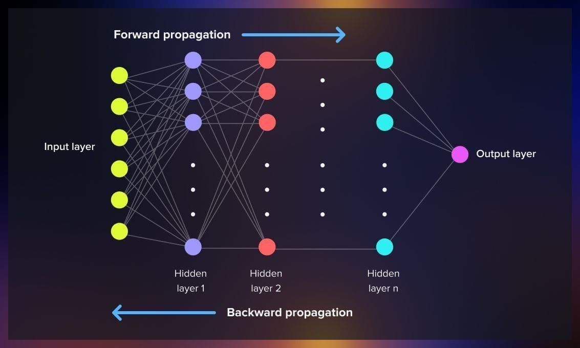
The algorithm for a given layer l during the backward pass follows a consistent pattern:

1. Receive Gradient: It takes the gradient of the loss with respect to its output activations, dA[l]. (Or, more conveniently, the gradient with respect to its pre-activations, dZ[l]).
2. Propagate through Activation: It calculates dZ[l] by multiplying dA[l] with the local gradient of the activation function, g'(Z[l]). This step effectively scales the error based on how "active" the neuron was.
3. Compute Parameter Gradients: It uses dZ[l] and the activations from the previous layer, A[l-1], to compute the gradients for its own weights (dW[l]) and biases (db[l]). These are the values we'll use to update the parameters.
4. Pass Gradient Backward: It calculates the gradient with respect to the previous layer's activations, dA[l-1], to continue the chain. This is done by propagating dZ[l] backward through the weights W[l].

By starting at the final layer and repeating this process in a loop, we can compute the gradients for the entire network.

2. Implementing Backpropagation for an L-Layer Network

Your preference for building things from scratch aligns perfectly with this task. We'll now study a fantastic, clear implementation that does exactly this using only Python and NumPy. This will serve as our primary guide for building our own backward method.

The video below implements a neural network with a configurable number of layers. We will focus specifically on the backward_propagation function.

Let's break down the implementation from the video into its key steps.

Step 1: The Starting Point (The Output Layer)

The backward pass begins at the very end of the network. We need to calculate the gradient of the loss function with respect to the pre-activation outputs of the last layer, dZ[L].

As you saw in the video and in our previous lesson's derivations, for common loss functions like Cross-Entropy (used for classification), this initial gradient has a very simple form:

Here:

• $A^{[L]}$ is the matrix of predictions from the forward pass.
• $Y$ is the matrix of true labels (one-hot encoded).

This simple subtraction gives us the initial error signal that we will propagate backward. The video code starts with this calculation at 00:27:56.

Step 2: Gradients for the Last Layer's Parameters (dW[L], db[L])

Once we have dZ[L], we can immediately compute the gradients for the weights and biases of the final layer, L. The formulas are:

• m is the number of training examples.
• $A^{[L-1]}$ are the activations from the previous layer, which were cached during the forward pass. Notice the transpose, which is crucial for the matrix multiplication dimensions to align correctly.

The video implements this at 00:28:05.

Step 3: The Backward Loop

This is the core of a deep learning implementation. We loop from layer L-1 down to layer 1. In each iteration, we compute the gradients for that layer.

The most important calculation is propagating the gradient from layer l+1 back to layer l. This is the vectorized chain rule in action:

Let's dissect this:

1. (W^{[l+1]})^T \cdot dZ^{[l+1]}: This part takes the gradient from the "next" layer (dZ[l+1]) and propagates it backward through that layer's weights (W[l+1]). The transpose ensures the shapes match up, effectively mapping the error contributions back to the neurons of the current layer l.
2. * g'(Z^{[l]}): This is an element-wise multiplication (Hadamard product). It scales the backpropagated gradient by the local gradient of the current layer's activation function. This is where the derivative of ReLU, sigmoid, or tanh comes into play.

After computing dZ[l], we can use the same formulas as in Step 2 to find dW[l] and db[l], since we now have the necessary dZ[l] and have already cached A[l-1].

The video's for loop, which starts around 00:29:45, masterfully implements this iterative process.

3. An Alternative Code Structure

The approach in the video—separating forward_propagation, backward_propagation, and update_parameters into distinct functions—is very clean and pedagogically sound. However, in object-oriented programming, it's also common to encapsulate this logic within a class.

The following resource shows an alternative but equally valid implementation structured within a NeuralNetwork class.

Seeing these different-but-equivalent structures is valuable, as it prepares you to read and understand various ML codebases you will encounter.

Conclusion

Congratulations! You have now dissected the implementation of the most critical algorithm in training neural networks. We've taken the mathematical formulas from our last session and mapped them directly to a flexible, from-scratch NumPy implementation.

Key Takeaways:

• Backpropagation is iterative: It starts with a simple gradient calculation at the output layer (dZ[L] = A[L] - Y) and then loops backward.
• The Core Calculation: In each step of the loop, the key is to compute dZ[l] for the current layer using the weights and dZ from the next layer (l+1).
• Chain Rule in Code: The formula dZ[l] = (W[l+1].T @ dZ[l+1]) * g'(Z[l]) is the chain rule expressed in vectorized NumPy operations.
• Parameter Gradients: Once dZ[l] is known, the gradients for that layer's parameters, dW[l] and db[l], are computed using dZ[l] and the activations from the previous layer, A[l-1].

Preview of the Next Lesson:
Our MLP can now compute all the gradients it needs. But with all these matrix transpositions and multiplications, it's very easy to introduce a subtle bug. A tiny error in the gradient calculation can silently prevent the network from learning, a notoriously difficult problem to debug. In our next lesson, we will implement gradient checking, a powerful technique to numerically verify that our backpropagation code is mathematically correct.