Batch Forward Propagation in MLPs

1. What is a Multi-Layer Perceptron (MLP)?

A Multi-Layer Perceptron is a type of feedforward neural network. It consists of:

1. An Input Layer, which receives the raw data.
2. One or more Hidden Layers, which perform intermediate computations and feature extraction.
3. An Output Layer, which produces the final prediction.

The "feedforward" part means that information flows in one direction—from input to output—without any loops.

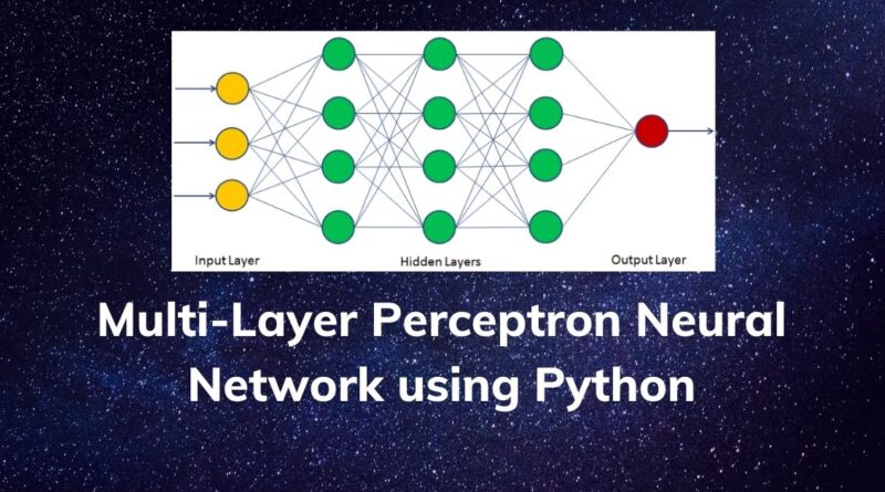
The power of MLPs comes from stacking these layers. The first layer might learn to recognize simple patterns (like edges or corners in an image), subsequent layers combine these to form more complex features (like eyes or noses), and the final layer uses these high-level features to make a classification.

For a conceptual overview of this layered structure, the following article is a helpful reference.

2. The Mechanics of a Single Layer Forward Pass

Let's break down what happens inside a single layer when data passes through it. The process involves two steps: a linear transformation followed by a non-linear activation.

For a batch of m input samples, your input data A_prev (activations from the previous layer) will be a matrix of shape (n_prev, m), where n_prev is the number of neurons in the previous layer.

1. Linear Step: We compute a weighted sum of the inputs and add a bias. This is an affine transformation.
   $Z=W\cdot A_{\text{prev}}+b$

   • $W$: The weight matrix for the current layer, with shape (n_current, n_prev).
   • $b$: The bias vector for the current layer, with shape (n_current, 1). NumPy's broadcasting handles adding this vector to each of the m columns of the W \cdot A_prev product.
   • $Z$: The result of the linear step, a matrix of shape (n_current, m).

2. Activation Step: We apply an element-wise activation function $g$ (like ReLU) to the result of the linear step.
   $A_{\text{current}}=g(Z)$

   • $A_{\text{current}}$: The output (activations) of the current layer, with shape (n_current, m). This becomes the input for the next layer.

This video provides an excellent visualization of how matrix multiplication efficiently performs these calculations for batches of data.

3. Implementing the Forward Pass: A Modular Approach

To keep our code clean, modular, and reusable, we'll follow an object-oriented approach. First, we'll create a DenseLayer class, and then an MLP class to manage the sequence of layers. This design mirrors how professional deep learning frameworks are structured.

We will rely on the initialize_parameters function you created in the last lesson. Let's assume you have it in a file named initialization.py or defined in the same notebook.

3.1. Building a Single DenseLayer

Let's start by creating a class to represent one dense layer. It will encapsulate its own weights, biases, and activation function.

import numpy as np
# Assuming your initialize_parameters function is available
# from initialization import initialize_parameters

# For demonstration, let's redefine the required functions here.
def initialize_parameters(model_shape, initialization_method='he'):
    parameters = {}
    L = len(model_shape)
    for l in range(1, L):
        parameters['b' + str(l)] = np.zeros((model_shape[l], 1))
        fan_in = model_shape[l-1]
        if initialization_method == 'xavier':
            scale = np.sqrt(1. / fan_in)
        else: # Default to 'he'
            scale = np.sqrt(2. / fan_in)
        parameters['W' + str(l)] = np.random.randn(model_shape[l], fan_in) * scale
    return parameters
    
def relu(Z):
    return np.maximum(0, Z)

def sigmoid(Z):
    return 1 / (1 + np.exp(-Z))

class DenseLayer:
    def __init__(self, n_input, n_output, activation='relu', init_method='he'):
        """
        Initializes a single dense layer.
        
        Args:
            n_input (int): Number of neurons in the previous layer (fan-in).
            n_output (int): Number of neurons in this layer.
            activation (str): 'relu' or 'sigmoid'.
            init_method (str): 'he' or 'xavier'.
        """
        # Initialize parameters using a helper function
        params = initialize_parameters([n_input, n_output], init_method)
        self.W = params['W1']
        self.b = params['b1']
        
        if activation == 'relu':
            self.activation_func = relu
        elif activation == 'sigmoid':
            self.activation_func = sigmoid
        
        self.cache = None # Will store values for backpropagation

    def forward(self, A_prev):
        """
        Performs the forward pass for this layer.
        
        Args:
            A_prev (np.array): Activations from the previous layer, shape (n_input, m_samples).
            
        Returns:
            A_current (np.array): Activations of the current layer, shape (n_output, m_samples).
        """
        # 1. Linear step
        Z = np.dot(self.W, A_prev) + self.b
        
        # 2. Activation step
        A_current = self.activation_func(Z)
        
        # Store values needed for backpropagation
        self.cache = (A_prev, self.W, self.b, Z)
        
        return A_current

Notice that we are storing (A_prev, W, b, Z) in a cache. This is a crucial design choice. While not used in the forward pass, these values are exactly what we'll need for the backpropagation algorithm in our next lesson.

3.2. Stacking Layers into an MLP

Now that we have a DenseLayer class, we can create an MLP class that acts as a container and orchestrates the forward pass through all the layers.

The logic is simple: the output of one layer becomes the input to the next.

Inspired by that structure, let's implement our MLP class.

class MLP:
    def __init__(self):
        self.layers = []

    def add_layer(self, layer):
        """Adds a DenseLayer object to the network."""
        self.layers.append(layer)

    def forward(self, X):
        """
        Performs the forward pass for the entire network.
        
        Args:
            X (np.array): Input data, shape (n_features, m_samples).
            
        Returns:
            A_final (np.array): Output of the final layer, shape (n_output_final, m_samples).
        """
        A = X
        for layer in self.layers:
            A = layer.forward(A)
        return A

4. Putting It All Together

We now have all the components to build and run an MLP. Let's create a network for a hypothetical binary classification problem with 4 input features. We'll use a 2-layer network: one hidden layer with 5 neurons (ReLU activation) and one output layer with 1 neuron (Sigmoid activation, suitable for binary classification).

# Create a batch of 10 samples with 4 features each
# Shape: (num_features, num_samples) -> (4, 10)
X_sample = np.random.randn(4, 10)

# 1. Instantiate the MLP
my_mlp = MLP()

# 2. Add layers
# Hidden Layer: 4 inputs -> 5 outputs, ReLU activation
my_mlp.add_layer(DenseLayer(n_input=4, n_output=5, activation='relu', init_method='he'))
# Output Layer: 5 inputs -> 1 output, Sigmoid activation
my_mlp.add_layer(DenseLayer(n_input=5, n_output=1, activation='sigmoid', init_method='xavier'))

# 3. Perform the forward pass
predictions = my_mlp.forward(X_sample)

# Print the shapes to verify
print("Input shape:", X_sample.shape)
print("Output/Predictions shape:", predictions.shape)
print("\nSample predictions (first 5):")
print(predictions[0, :5])

If you run this code, you should see that the output shape is (1, 10), meaning we got one prediction for each of the 10 samples in our batch, which is exactly what we want. The prediction values will be between 0 and 1 due to the final sigmoid activation.

Conclusion

Congratulations! You have successfully implemented one of the most fundamental algorithms in deep learning. You've brought together parameter initialization and activation functions to build a complete forward pass for a multi-layer perceptron that can efficiently process batches of data.

Key Takeaways:

• An MLP processes information by passing it sequentially through a series of layers (input, hidden, output).
• Each layer performs a linear transformation (Z = WX + b) followed by a non-linear activation (A = g(Z)).
• Using matrix multiplication is the key to efficient batch processing, allowing the network to process many samples at once.
• A modular, object-oriented design (DenseLayer, MLP classes) makes the code clean and scalable.
• Storing intermediate values (A_prev, W, b, Z) in a cache during the forward pass is essential for the next step: training.

Preview of the Next Lesson:
Our network can now make predictions, but they are completely random because the weights have not been trained. The next big question is: how do we adjust these weights to improve the predictions? This is the job of the backpropagation algorithm. In the next lesson, we will manually derive the gradients using the chain rule and begin implementing backpropagation, which uses the cache from our forward pass to calculate how to update every weight and bias in the network.