Weight Initialization Techniques

1. Why Initialization Matters: The Problem with Naive Approaches

In the previous lesson, we saw that activation functions like Sigmoid and Tanh "saturate" (their gradients approach zero) for large positive or negative inputs. If we're not careful, our initial weights could immediately push neuron outputs into these saturation zones, causing the learning process to grind to a halt before it even begins. This is the vanishing gradient problem. Conversely, weights that are too large can cause outputs to grow uncontrollably layer by layer, leading to numerical instability and the exploding gradient problem.

So, what are our options?

• Zero Initialization: Initializing all weights to zero. This is a non-starter. If all weights are the same, all neurons in a layer will learn the exact same features. The network fails to break symmetry and its capacity is severely limited.
• Random Initialization: We can initialize weights to random values to break symmetry. But what is the right scale for these random numbers? Too small, and we risk vanishing gradients. Too large, and we risk exploding gradients.

To get a concise summary of these challenges, please watch the first few minutes of the following video.

As you can see, we need a more principled approach—one that sets the initial weights "just right".

2. The Core Idea: Scaling Weights by Network Architecture

The key insight, developed by researchers, is that the variance of the weights should be dependent on the number of connections a neuron receives. We refer to the number of incoming connections to a neuron as its fan-in and the number of outgoing connections as its fan-out.

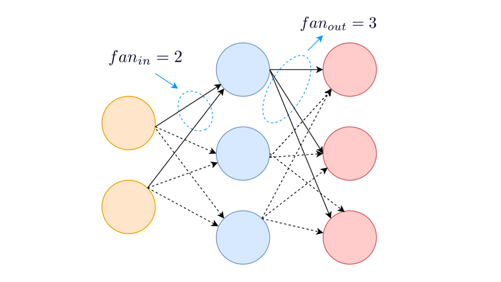
The intuition is as follows: if a neuron has a large fan_in, it sums many weighted inputs. To prevent this sum from becoming too large or small, the individual weights should be smaller. Conversely, if a neuron has a small fan_in, the weights can be larger.

Let's watch a short clip from Andrew Ng that builds this intuition.

This principle of scaling the variance of weights inversely with the fan_in is the foundation of modern initialization techniques. Let's implement the two most important ones.

3. Xavier (or Glorot) Initialization

Proposed by Xavier Glorot and Yoshua Bengio in 2010, this strategy is designed to work well with activation functions that are zero-centered and saturate, like Tanh and Sigmoid. It aims to keep the variance of activations and gradients constant across all layers.

For a layer's weights, we sample from a normal distribution with a mean of 0 and a specific variance:

$\text{Var}(W)=\frac{1}{n_{in}}$

where $n_{in}$ is the fan-in of the layer. To implement this, we draw weights from a standard normal distribution (mean 0, variance 1) and scale them by $\sqrt{\frac{1}{n_{in}}}$.

Implementation

Your task is to write a function that initializes the parameters for a neural network. We'll build a single function that can handle multiple initialization methods.

The following resource provides a great template for an initialize_parameters function. We will use its structure to build our own.

Now, let's write the code for random and Xavier initialization. The weights $W^{[l]}$ for layer $l$ will have the shape (size of layer l, size of layer l-1). The fan_in is therefore the size of the previous layer, model_shape[l-1].

import numpy as np

def initialize_parameters(model_shape, initialization_method='he'):
    """
    Initializes parameters W and b for a network.
    
    Arguments:
    model_shape -- list containing the dimensions of each network layer (e.g., [784, 256, 128, 10])
    initialization_method -- string, one of 'random', 'xavier', or 'he'
    
    Returns:
    parameters -- dictionary containing weight (W) and bias (b) parameters for each layer
    """
    parameters = {}
    L = len(model_shape) # Number of layers in the network

    for l in range(1, L):
        # Biases are always initialized to zero
        parameters['b' + str(l)] = np.zeros((model_shape[l], 1))
        
        # Get the fan-in (number of neurons in the previous layer)
        fan_in = model_shape[l-1]

        if initialization_method == 'random':
            # Simple scaled random initialization
            parameters['W' + str(l)] = np.random.randn(model_shape[l], fan_in) * 0.01
        
        elif initialization_method == 'xavier':
            # Xavier initialization
            scale_factor = np.sqrt(1. / fan_in)
            parameters['W' + str(l)] = np.random.randn(model_shape[l], fan_in) * scale_factor
            
    return parameters

# Example usage:
# A network with 784 inputs, a hidden layer of 256 neurons, and a 10-neuron output layer.
layer_dims = [784, 256, 10]
params_xavier = initialize_parameters(layer_dims, initialization_method='xavier')

# Let's check the standard deviation of the weights for the first layer
print(f"Xavier: Std dev of W1: {np.std(params_xavier['W1'])}")
print(f"Expected std dev: {np.sqrt(1./784):.4f}")

Notice that we also have a "random" method which multiplies by a small constant (0.01). Xavier improves upon this by making the scaling factor dynamic based on the layer's architecture.

4. He Initialization

While Xavier works well for Tanh and Sigmoid, it's not optimal for the ReLU activation function. Because ReLU sets all negative inputs to zero, it effectively "kills" about half of the neuron outputs, which changes the variance of the activations.

Kaiming He et al. proposed a modification in 2015 specifically for ReLU-based networks. The formula is a minor but crucial adjustment to Xavier's:

$\text{Var}(W)=\frac{2}{n_{in}}$

The implementation simply changes the scaling factor to $\sqrt{\frac{2}{n_{in}}}$. This slightly larger scale compensates for the variance lost when ReLU zeroes out negative values.

Let's watch a quick explanation of the He initialization formula.

Implementation

Now it's your turn to complete our function.

import numpy as np

def initialize_parameters(model_shape, initialization_method='he'):
    """
    Initializes parameters W and b for a network.
    
    Arguments:
    model_shape -- list containing the dimensions of each network layer (e.g., [784, 256, 128, 10])
    initialization_method -- string, one of 'random', 'xavier', or 'he'
    
    Returns:
    parameters -- dictionary containing weight (W) and bias (b) parameters for each layer
    """
    parameters = {}
    L = len(model_shape)

    for l in range(1, L):
        parameters['b' + str(l)] = np.zeros((model_shape[l], 1))
        
        fan_in = model_shape[l-1]

        if initialization_method == 'random':
            parameters['W' + str(l)] = np.random.randn(model_shape[l], fan_in) * 0.01
        
        elif initialization_method == 'xavier':
            scale_factor = np.sqrt(1. / fan_in)
            parameters['W' + str(l)] = np.random.randn(model_shape[l], fan_in) * scale_factor
            
        elif initialization_method == 'he':
            # He initialization
            scale_factor = np.sqrt(2. / fan_in)
            parameters['W' + str(l)] = np.random.randn(model_shape[l], fan_in) * scale_factor
            
    return parameters

# Example usage for He initialization:
layer_dims = [784, 256, 10]
params_he = initialize_parameters(layer_dims, initialization_method='he')

# Let's check the standard deviation of the weights for the first layer
print(f"He: Std dev of W1: {np.std(params_he['W1'])}")
print(f"Expected std dev: {np.sqrt(2./784):.4f}")

You now have a flexible function that can initialize a network's weights using the most appropriate strategy based on the activation functions you plan to use. This is a critical piece of the puzzle for building and training your neural network from scratch.

Conclusion

In this lesson, you've moved from the "what" (activation functions) to the "how to start" (weight initialization). You've seen that a thoughtful initialization strategy is not an optional tweak but a requirement for successfully training deep networks. By implementing random, Xavier, and He initialization, you now have the tools to set your network up for success.

Key Takeaways:

• Initialization is Critical: Naive weight initialization can lead to vanishing or exploding gradients, preventing a network from learning.
• Symmetry Must Be Broken: Initializing weights to the same value (e.g., zero) is a critical error. Random initialization is necessary.
• Xavier Initialization: Best for tanh and sigmoid activations. It scales the variance of weights by $\frac{1}{n_{in}}$.
• He Initialization: The standard for ReLU activations. It scales the variance of weights by $\frac{2}{n_{in}}$ to account for ReLU's behavior.
• Rule of Thumb: Use He initialization for layers with ReLU activations and Xavier initialization for layers with Tanh activations.

Preview of the Next Lesson:
You've now implemented two of the three core components of a neuron layer: the activation function and the parameter initialization. The final piece is combining them. In the next lesson, you will implement the forward propagation algorithm for a multi-layer perceptron (MLP). This is where we'll put everything together and see, for the first time, how data flows from the input layer through the hidden layers to produce an output.