Implementing Dropout in the Forward Pass

1. Understanding Overfitting and Dropout

An overfitted model performs exceptionally well on the data it was trained on but fails to generalize to new, unseen data. It essentially memorizes the training set's noise and idiosyncrasies rather than learning the underlying patterns.

Dropout combats this by introducing a form of randomness during training. At each training step, it randomly "drops out" (i.e., temporarily deactivates) a fraction of the neurons in a layer.

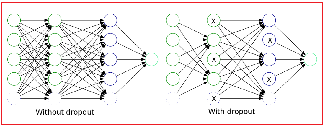
By training on a different "thinned" network for each mini-batch, dropout prevents neurons from becoming too dependent on each other. This forces the network to learn more robust features that are useful in a variety of contexts, leading to better performance on unseen data.

To get a solid conceptual grasp of this, let's watch a short video.

2. Implementing Dropout: The Mask and Scale Method

Instead of actually resizing weight matrices, which would be computationally inefficient, we can simulate dropout using a binary mask. This is the standard approach. For each layer that has dropout enabled during a forward pass in training, we perform two steps:

1. Create a Mask: Generate a random matrix of the same dimensions as the layer's activation output, A. We then create a binary mask by checking where the random values are less than a keep_prob hyperparameter. keep_prob is the probability that a neuron is kept active (e.g., keep_prob=0.8 means 20% of neurons are dropped).
2. Apply the Mask: Multiply the activations A element-wise by this binary mask. This effectively sets the output of the dropped neurons to zero.

The Need for Scaling: Inverted Dropout

There's one crucial detail. If we drop 20% of neurons during training, the total output of that layer is, on average, 20% smaller than it would be during testing (when all neurons are active). This creates a mismatch between training and inference.

To fix this, we use a technique called inverted dropout. During training, after applying the dropout mask, we scale up the activations of the remaining neurons by dividing by keep_prob.

$A_{\text{dropout}}=\frac{A_{\text{masked}}}{keep\_prob}$

This ensures that the expected output of the layer remains the same during both training and testing. The great advantage is that we don't need to make any changes to our network during inference—we simply use all the neurons as is.

The following article provides a very clear "from scratch" implementation of this exact concept.

3. Modifying Our MLP for Dropout

Now, let's integrate what we've learned into the DenseLayer and MLP classes from our previous lesson.

The key changes will be:

• The DenseLayer will be initialized with a keep_prob parameter.
• The forward method in DenseLayer will be updated to apply the inverted dropout logic. It will only do this during training.
• The cache will be updated to store the dropout mask D, as we will need it for backpropagation later.
• The MLP's forward method will accept a training flag to pass down to its layers.

Here are the updated classes. Note the modifications, especially within the DenseLayer's __init__ and forward methods.

import numpy as np

# Let's keep the helper functions from the previous lesson
def relu(Z):
    return np.maximum(0, Z)

def sigmoid(Z):
    return 1 / (1 + np.exp(-Z))

def initialize_parameters(model_shape, initialization_method='he'):
    parameters = {}
    L = len(model_shape)
    for l in range(1, L):
        parameters['b' + str(l)] = np.zeros((model_shape[l], 1))
        fan_in = model_shape[l-1]
        if initialization_method == 'xavier':
            scale = np.sqrt(1. / fan_in)
        else: # Default to 'he'
            scale = np.sqrt(2. / fan_in)
        parameters['W' + str(l)] = np.random.randn(model_shape[l], fan_in) * scale
    return parameters

class DenseLayer:
    def __init__(self, n_input, n_output, activation='relu', init_method='he', keep_prob=1.0):
        """
        Initializes a single dense layer with dropout capability.
        
        Args:
            n_input (int): Number of neurons in the previous layer.
            n_output (int): Number of neurons in this layer.
            activation (str): 'relu' or 'sigmoid'.
            init_method (str): 'he' or 'xavier'.
            keep_prob (float): Probability of keeping a neuron active during dropout.
                               1.0 means no dropout.
        """
        params = initialize_parameters([n_input, n_output], init_method)
        self.W = params['W1']
        self.b = params['b1']
        
        if activation == 'relu':
            self.activation_func = relu
        elif activation == 'sigmoid':
            self.activation_func = sigmoid
            
        self.keep_prob = keep_prob
        self.cache = None

    def forward(self, A_prev, training=False):
        """
        Performs the forward pass for this layer.
        
        Args:
            A_prev (np.array): Activations from the previous layer, shape (n_input, m_samples).
            training (bool): Flag to indicate if the model is in training mode.
            
        Returns:
            A (np.array): Activations of the current layer, shape (n_output, m_samples).
        """
        Z = np.dot(self.W, A_prev) + self.b
        A = self.activation_func(Z)
        
        D = None # Initialize dropout mask
        if training and self.keep_prob < 1.0:
            # 1. Create a dropout mask D
            D = np.random.rand(A.shape[0], A.shape[1]) < self.keep_prob
            # 2. Apply mask to shut down neurons
            A = A * D
            # 3. Scale the remaining neurons (Inverted Dropout)
            A = A / self.keep_prob
            
        # Store values needed for backpropagation
        # Note: We now store D in the cache as well!
        self.cache = (A_prev, self.W, self.b, Z, D)
        
        return A

class MLP:
    def __init__(self):
        self.layers = []

    def add_layer(self, layer):
        self.layers.append(layer)

    def forward(self, X, training=False):
        """
        Performs the forward pass for the entire network.
        
        Args:
            X (np.array): Input data, shape (n_features, m_samples).
            training (bool): Flag to indicate if the model is in training mode.
            
        Returns:
            A_final (np.array): Output of the final layer.
        """
        A = X
        for layer in self.layers:
            # Pass the training flag to each layer
            A = layer.forward(A, training=training)
        return A

4. Observing Dropout in Action

Let's build the same network as last time, but now with dropout in the hidden layer (keep_prob=0.8). We'll perform a forward pass in both training and inference mode to see the difference.

# Create a batch of 5 samples with 4 features each
X_sample = np.random.randn(4, 5)

# 1. Instantiate the MLP
my_dropout_mlp = MLP()

# 2. Add layers with dropout
# Hidden Layer: 5 neurons, ReLU activation, 20% dropout (keep_prob=0.8)
my_dropout_mlp.add_layer(DenseLayer(n_input=4, n_output=5, activation='relu', keep_prob=0.8))
# Output Layer: 1 neuron, Sigmoid activation, no dropout
my_dropout_mlp.add_layer(DenseLayer(n_input=5, n_output=1, activation='sigmoid'))

# 3. Forward pass in TRAINING mode
print("--- Training Mode (Dropout ON) ---")
# Set a seed for reproducibility of the random mask
np.random.seed(42) 
predictions_train = my_dropout_mlp.forward(X_sample, training=True)

# Let's inspect the activations of the first layer
hidden_activations_train = my_dropout_mlp.layers[0].activation_func(my_dropout_mlp.layers[0].cache[3])
print("Hidden activations BEFORE dropout:\n", hidden_activations_train)

dropout_mask = my_dropout_mlp.layers[0].cache[4]
print("\nDropout mask (1s are kept, 0s are dropped):\n", dropout_mask.astype(int))

final_hidden_activations = my_dropout_mlp.layers[0].forward(X_sample, training=True)
print("\nHidden activations AFTER dropout and scaling:\n", final_hidden_activations)


# 4. Forward pass in INFERENCE mode
print("\n--- Inference Mode (Dropout OFF) ---")
predictions_inference = my_dropout_mlp.forward(X_sample, training=False)
final_hidden_activations_inference = my_dropout_mlp.layers[0].forward(X_sample, training=False)
print("Hidden activations during inference (all active):\n", final_hidden_activations_inference)

When you run this code, you'll see that in training mode, some of the hidden activations are zeroed out by the mask. The non-zero values are scaled up. In inference mode, all activations are present and unscaled. This clearly demonstrates the different behaviors.

Conclusion

You have now successfully integrated dropout, a key regularization technique, into your neural network's forward pass. This is a critical step towards building robust models that generalize well to new data.

Key Takeaways:

• Dropout is a regularization method that fights overfitting by randomly deactivating neurons during training.
• It is implemented efficiently using a binary mask and element-wise multiplication.
• Inverted Dropout is the standard practice where activations are scaled up during training (/ keep_prob). This simplifies the inference phase, as no modifications are needed.
• A training flag is essential to control the model's behavior, ensuring dropout is only active when learning.
• The dropout mask must be cached during the forward pass, as it's required for backpropagation.

Preview of the Next Lesson:
Our network can now make predictions and even regularize itself during training. However, it still can't learn. The next step is to figure out how to update the weights based on prediction errors. This process is called backpropagation. In the next lesson, we will begin our journey into training by manually deriving the gradients for a simple two-layer network using the chain rule. This will lay the mathematical foundation for implementing the full backpropagation algorithm.