Reading Topography: Slope and Relief

1. Understanding Relief

Before we tackle slope, let's start with a related and more straightforward concept: relief.

In geography, relief refers to the difference in elevation between the highest and lowest points within a given area on a map. It gives you a quick measure of how flat or mountainous the terrain is.

As you've just read, the key points are:

• Height is local: the elevation difference between the base and summit of a single feature (e.g., a 200 ft high hill).
• Relief is regional: the elevation difference between the absolute highest and lowest points on the entire map or a defined area.

How to Calculate Relief

Calculating relief is a simple subtraction:
Relief = Highest Elevation - Lowest Elevation

1. Find the highest point: Look for the highest index contour, a labeled summit (often marked with a triangle or 'X' and an elevation number), or the highest closed contour loop. Remember from our last lesson, the area inside the highest contour line is higher still, but less than the next potential contour.
2. Find the lowest point: Look for the lowest index contour or the lowest elevation marked on the map, often along a river or at the edge of the map area.
3. Calculate the difference: Subtract the lowest value from the highest value.

For example, if the highest peak on a map is 1,245 meters and the lowest point in a valley is 300 meters, the total relief of that map area is 1,245 - 300 = 945 meters. This would be considered 'moderate' to 'high' relief.

2. Describing Slope: Beyond "Steep" and "Gentle"

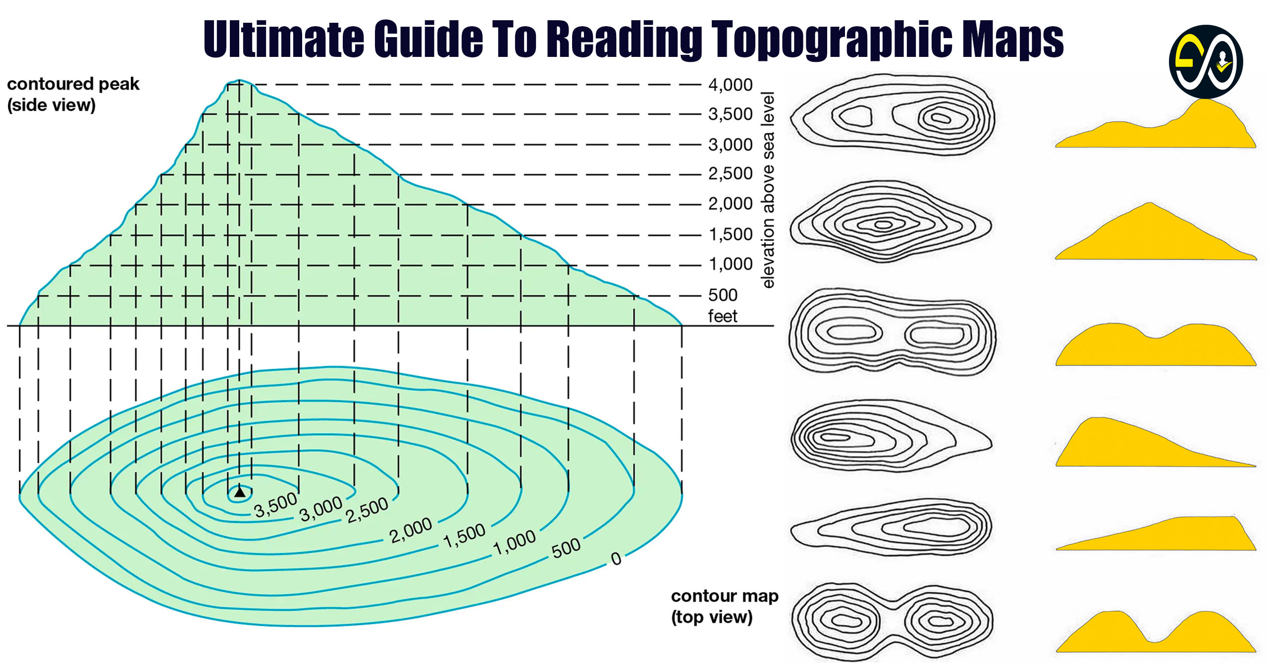
In our last lesson, you learned the fundamental rule: the closer the contour lines, the steeper the slope. Now, let's add more nuance. Slopes aren't always uniform; they can change their steepness. The two main variations are concave and convex slopes.

To summarize the video's key points:

• Concave Slope: The slope is gentle at the bottom and gets steeper towards the top. On a map, the contour lines are widely spaced at the bottom and become closely packed at the top. (Remember the 'A' mnemonic from the video: wide at the bottom, narrow at the top).
• Convex Slope: The slope is steep at the bottom and gets gentler towards the top. On a map, the contour lines are closely packed at the bottom and become widely spaced at the top. (Remember the 'V' mnemonic).

3. Calculating Slope: The Gradient

Describing a slope as "steep" or "concave" is useful, but often we need to be more precise. We can do this by calculating the gradient of the slope.

The gradient is a numerical measure of a slope's steepness. It is expressed as the ratio of the vertical change in elevation (the "rise") to the horizontal distance (the "run").

The formula is:

Since you have a background in basic calculus, you might recognize this as being very similar to the definition of a derivative ($dy/dx$), which measures an instantaneous rate of change. Here, we are calculating the average slope between two specific points.

Let's watch a video that walks through a practical example of this calculation.

Step-by-Step Guide to Calculating Gradient

Let's break down the process you just saw:

Step 1: Find the Vertical Interval (VI or Rise)
This is the difference in elevation between your starting and ending points. You find this by reading the contour lines.
Example: If you are moving from a contour line at 100m to one at 150m, your VI is 50m.

Step 2: Find the Horizontal Distance (HD or Run)
This requires two parts:

1. Measure the straight-line distance on the map between your two points (e.g., in centimeters).
2. Use the map's scale to convert this map distance into the real-world ground distance (e.g., in meters). (This is a skill from our lesson on map scale!)

Example: You measure 2 cm on the map. The map scale is 1:50,000, which means 1 cm on the map equals 50,000 cm (or 500 m) on the ground. Your HD is 2 cm x 500 m/cm = 1,000 m.

Step 3: Calculate and Express the Gradient
Divide the VI by the HD. Crucially, make sure both are in the same units.

Example: Using the values above:

This gradient can be expressed in several ways:

• As a fraction: 1/20
• As a ratio: 1:20
• Verbally: "A rise of 1 in 20." This means for every 20 meters you travel horizontally, your elevation increases by 1 meter.

The smaller the second number in the ratio, the steeper the slope. A gradient of 1:5 is much steeper than a gradient of 1:50.

4. Application: Identifying Features on a Map

Now, let's bring all these concepts together—relief, slope types, and landforms—by looking at a complete topographic map.

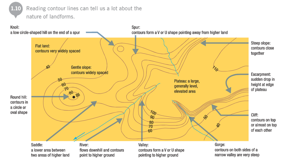
Observe how:

• Steep slopes and cliffs have tightly packed or touching contours.
• Gentle slopes and flat land have widely spaced contours.
• Valleys and gorges show V-shaped contours pointing uphill.
• Spurs show U- or V-shaped contours pointing downhill.
• A saddle is a low area between two high points (knolls).

By combining your knowledge of landform shapes (from the last lesson) with your new ability to interpret relief and slope, you can build a very detailed mental model of the landscape from the map alone.

Conclusion

Today we added a crucial quantitative layer to your map-reading skills. You've moved beyond a purely visual interpretation to one that includes precise measurement and calculation.

Key Takeaways:

• Relief is the difference between the highest and lowest elevations on a map, giving a sense of the overall ruggedness of the terrain.
• Slopes can be not only steep or gentle but also concave (steepening uphill) or convex (flattening uphill), each with a distinct contour pattern.
• Gradient is the numerical representation of a slope, calculated as Rise / Run and expressed as a ratio (e.g., 1:10).
• Calculating gradient requires finding the vertical interval from the contours and the horizontal distance using the map scale.

Preview of the Next Lesson:
We've spent the last few lessons focused on representing the 3D elevation of the land on a 2D map. But this raises a more fundamental question: how do we represent the curved, spherical surface of the entire Earth on a flat piece of paper? In our next lesson, we will tackle this challenge by exploring the topic of map projections. You will learn why every flat map of the world is distorted in some way and how cartographers choose different projections to preserve different properties like shape, area, or distance.