WKB Approximation in Quantum Mechanics

Welcome to our next lesson. In our previous session, we explored how to find asymptotic expansions for integrals using the stationary phase and steepest descent methods. We saw that by deforming contours in the complex plane, we could isolate the dominant contributions to an integral and systematically build an approximation. Today, we will apply a very similar intellectual framework, but instead of an integral, we will attack an operator equation: the time-independent Schrödinger equation.

This leads us to the Wentzel-Kramers-Brillouin (WKB) approximation, a cornerstone of semiclassical physics. We will treat Planck's constant, $ℏ$ , as a small parameter and seek an asymptotic expansion for the wavefunction. This method provides powerful physical intuition, connecting quantum mechanics back to its classical roots, and delivers excellent approximations for energy levels and quantum tunnelling rates. We will see how the ideas of stationary phase and asymptotic series, which you are now familiar with, manifest themselves in the solutions to this fundamental equation.

1. The Semiclassical Ansatz

The core idea of the WKB method is to find solutions to the Schrödinger equation in regimes where the potential $V (x)$ varies slowly. What does "slowly" mean? Intuitively, it means the potential doesn't change much over the length scale of a quantum particle's wavefunction, its de Broglie wavelength.

To formalize this, we first recall the time-independent Schrödinger equation in one dimension:

- \frac{ℏ ^{2}}{2 m} \frac{d ^{2} ψ}{d x ^{2}} + V (x) ψ = E ψ

It's useful to rearrange this into a more suggestive form:

\frac{d ^{2} ψ}{d x ^{2}} + \frac{2 m}{ℏ ^{2}} (E - V (x)) ψ = 0

We can define a position-dependent "local momentum" $p (x)$ , which is what a classical particle's momentum would be at position $x$ :

p (x) = 2 m (E - V (x))

Using this, the Schrödinger equation becomes:

ℏ^{2} \frac{d ^{2} ψ}{d x ^{2}} + p (x)^{2} ψ = 0

This equation connects the curvature of the wavefunction to the classical momentum at that point. To get a feel for the physical ideas behind the WKB approximation, the following video provides an excellent introduction.

L6.5 Semiclassical approximation and local de Broglie wavelength

This video from MIT OpenCourseWare introduces the physical context for the WKB approximation. It frames the problem in terms of a slowly varying de Broglie wavelength and treats \hbar as a small expansion parameter.

Please watch the first part of the video from the beginning, which gives the historical context. Then, focus on the segment from local momentum, where the lecturer introduces the concept of a position-dependent momentum p(x) and wavelength \lambda(x), and recasts the Schrödinger equation in this "semiclassical language."

Inspired by the oscillatory nature of wavefunctions and our work with phase integrals in the last lesson, we make the WKB ansatz for the solution:

ψ (x) = e^{i S (x) /ℏ}

Here, $S (x)$ is a complex function we need to determine. The real part of $S (x)$ governs the phase of $ψ$ , while its imaginary part governs the amplitude. Plugging this into the rearranged Schrödinger equation gives a nonlinear differential equation for $S (x)$ :

(S^{'} (x))^{2} - i ℏ S^{''} (x) = p (x)^{2}

This equation is exact. We've traded a linear equation for $ψ$ for a nonlinear one for $S$ . The benefit is that this new equation is perfectly structured for an asymptotic expansion in the small parameter $ℏ$ . We expand $S (x)$ as a power series in $ℏ$ :

S (x) = S_{0} (x) + ℏ S_{1} (x) + ℏ^{2} S_{2} (x) + \dots

Substituting this series into the equation for $S$ and collecting terms order-by-order in $ℏ$ gives a hierarchy of simpler equations. Let's look at the first two orders.

6. Approximation Methods

This text from David Tong's lecture notes provides a crisp derivation of the WKB expansion.

Please read the section "The Semi-Classical Expansion" from the beginning, down to this point. This will walk you through substituting the WKB ansatz into the Schrödinger equation and solving for the first two terms, W_0 (which is our S_0) and W_1 (our S_1).

Let's summarize the key results from that derivation:

Zeroth Order ( $ℏ^{0}$ ): $(S_{0}^{'})^{2} = p (x)^{2}$ . This gives $S_{0}^{'} (x) = \pm p (x)$ , so
$S_{0} (x) = \pm \int p (x^{'}) d x^{'}$
To leading order, the phase of the wavefunction accumulates based on the integral of the classical momentum. This integral is precisely the classical action for a particle moving from a reference point to $x$ .
First Order ( $ℏ^{1}$ ): $2 S_{0}^{'} S_{1}^{'} - i S_{0}^{''} = 0$ . This yields $S_{1}^{'} (x) = i \frac{p ^{'} ( x )}{2 p ( x )}$ , so
$S_{1} (x) = \frac{i}{2} ln p (x)$

Combining these terms, the wavefunction to this order is $ψ (x) \approx e^{i (S_{0} + ℏ S_{1}) /ℏ} = e^{i S_{0} /ℏ} e^{i S_{1}}$ . Substituting our solutions for $S_{0}$ and $S_{1}$ gives the celebrated WKB approximation:

ψ_{W K B} (x) \approx \frac{C _{\pm}}{p ( x )} exp (\pm \frac{i}{ℏ} \int^{x} p (x^{'}) d x^{'})

The general solution is a linear combination of these two. This single formula contains a wealth of physics. Notice the amplitude is proportional to $1/ p (x)$ . Since $∣ ψ (x) ∣^{2} \propto 1/ p (x)$ , the probability of finding the particle at $x$ is inversely proportional to its classical momentum there. This makes perfect intuitive sense: the particle is more likely to be found where it moves slowly.

The character of the solution depends on the sign of $E - V (x)$ :

Classically Allowed Region ( $E > V (x)$ ): Here, $p (x)$ is real. The solution is oscillatory, representing a propagating wave.
Classically Forbidden Region ( $E < V (x)$ ): Here, $p (x)$ is purely imaginary. Let's write $p (x) = i ∣ p (x) ∣$ . The solution becomes a real exponential, representing exponential decay or growth.

ψ_{W K B} (x) \approx \frac{C _{\pm}^{'}}{∣ p ( x ) ∣} exp (\pm \frac{1}{ℏ} \int^{x} ∣ p (x^{'}) ∣ d x^{'})

2. Breakdown at Turning Points: The Connection Problem

Like any approximation, the WKB method has a limited domain of validity. The expansion is valid when successive terms are smaller than the previous ones. This translates to the condition that the local de Broglie wavelength $λ (x) = 2 π ℏ/ p (x)$ must vary slowly.

[PDF] Quantum Physics III Chapter 3: Semiclassical Approximation

These notes by Barton Zwiebach for MIT's Quantum Physics III course give a detailed look at the validity condition.

Please read the section "Validity of the approximation". Focus on the derivation leading to the conditions d\lambda/dx \ll 1 and the equivalent statement that the change in potential over one wavelength should be much less than the kinetic energy.

This validity condition reveals a critical flaw. At a classical turning point, where $E = V (x)$ , the classical momentum $p (x)$ goes to zero. Consequently, the de Broglie wavelength $λ (x)$ diverges, and the validity condition $∣ d λ / d x ∣ ≪ 1$ is dramatically violated. Furthermore, the WKB wavefunction itself, with its $1/ p (x)$ factor, blows up at the turning point.

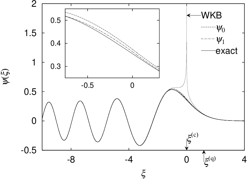
An exact solution $\psi(\xi)$ for a linear potential (solid line) compared with the zeroth-order ($\psi_0$, dashed) and first-order ($\psi_1$, dot-dashed) WKB approximations. The WKB solutions diverge at the turning point $\xi=0$, while the exact solution (an Airy function) smoothly connects the oscillatory region ($\xi < 0$) to the exponentially decaying region ($\xi > 0$).

So, what do we do? We have valid approximate solutions far from the turning point (the "outer" solutions), but they fail in the region around it (the "inner" region). This is a classic singular perturbation problem. The strategy is to find a different, more accurate approximation valid near the turning point, and then "match" it to our WKB solutions on either side.

Near a turning point $x_{0}$ , we can approximate the potential with its tangent line: $V (x) \approx E + V^{'} (x_{0}) (x - x_{0})$ . With this linear potential, the Schrödinger equation becomes the Airy equation, whose solutions are the Airy functions, Ai(u) and Bi(u). These functions provide the bridge that connects the oscillatory and exponential WKB solutions.

3. Applications: Quantization and Tunneling

The true power of the WKB method is revealed when we use these connection formulas to solve physical problems.

Bound States and Bohr-Sommerfeld Quantization

Consider a particle in a potential well with two turning points, $a$ and $b$ . Far to the left ( $x ≪ a$ ) and far to the right ( $x ≫ b$ ), the wavefunction must decay to zero. We therefore must pick the exponentially decaying WKB solutions in these regions. The connection formulas, derived from the asymptotic behavior of the Airy function, dictate the specific form of the oscillatory solution between the turning points.

For a consistent solution, the oscillatory wavefunction derived by connecting from the left turning point must match the one derived by connecting from the right. This consistency requirement can only be met for specific, discrete energy values. It leads to the famous Bohr-Sommerfeld quantization condition:

\int_{a}^{b} p (x^{'}) d x^{'} = (n + \frac{1}{2}) π ℏ, for n = 0, 1, 2, \dots

This remarkable formula determines the approximate energy levels of a quantum system using only an integral of the classical momentum over one period of classical motion. The fact that action is quantized in units of $ℏ$ is a profound semiclassical result.

6. Approximation Methods

This section of the notes by David Tong demonstrates the matching procedure across a potential well to derive the Bohr-Sommerfeld quantization condition.

Read the section "Bound State Spectrum", paying close attention to how the two different expressions for the wavefunction in the central region, Eqs. (6.24) and (6.25), are forced to be consistent. Then, review the application to the harmonic oscillator, a rare case where the WKB approximation coincidentally yields the exact energy spectrum.

Quantum Tunneling

Another classic application is calculating the probability of a particle tunneling through a potential barrier. Imagine a wave incident on a barrier from the left. Using the connection formulas, we can track the wavefunction across the barrier.

We start with the transmitted wave on the far right, which is purely right-moving.
We use the connection formula at the second turning point ( $x = b$ ) to find the wavefunction inside the barrier. It will be a combination of growing and decaying exponentials, but only the growing part (as we move left from $b$ ) can be reliably determined.
We continue this solution across the barrier to the first turning point ( $x = a$ ).
We use the connection formula at $x = a$ to find the incident and reflected waves on the left side.

The ratio of the probability current of the transmitted wave to that of the incident wave gives the transmission probability, $T$ . The result is dominated by an exponential factor:

T \approx exp (- \frac{2}{ℏ} \int_{a}^{b} ∣ p (x^{'}) ∣ d x^{'})

where the integral is over the classically forbidden region.

This exponential suppression is a generic feature of quantum tunneling. For you, as someone studying QFT, this formula has a deep and beautiful connection to instantons. The exponent is precisely $2 S_{E} /ℏ$ , where $S_{E}$ is the Euclidean action of a classical "bounce" solution (an instanton) that traverses the forbidden region in imaginary time. The WKB approximation for a simple particle gives a glimpse into the powerful path integral techniques used in field theory to calculate non-perturbative effects.

L7.2 Approximate WKB solutions

This MIT OCW video provides the details of constructing the WKB solutions and interpreting them.

First, watch the derivation of the S0 and S1 terms, which reconstructs the argument from the reading. Then, see how these are assembled into the full WKB solutions for both allowed and forbidden regions. Finally, watch the discussion on probability density and current from 13:59 to 19:01 to solidify the physical interpretation.

Conclusion

In this lesson, we have seen how to formulate and apply the WKB approximation, a powerful tool in the theoretical physicist's arsenal. It embodies the principle of asymptotic analysis applied directly to the Schrödinger equation.

Key Takeaways:

The WKB method is a semiclassical approximation that seeks an asymptotic solution to the Schrödinger equation in powers of $ℏ$ .
The ansatz $ψ (x) = e^{i S (x) /ℏ}$ leads to an expansion where the leading term $S_{0}$ is the classical action, connecting quantum phase to classical motion.
The amplitude of the WKB wavefunction, $∣ ψ ∣^{2} \propto 1/ p (x)$ , reflects the classical intuition that a particle is most likely to be found where it moves the slowest.
The approximation breaks down at classical turning points ( $p (x) = 0$ ), requiring a separate "inner" solution (the Airy function) to connect the "outer" WKB solutions across these points.
Applying these connection rules allows for the derivation of the Bohr-Sommerfeld quantization condition for bound states and the calculation of exponential suppression factors for quantum tunneling.

The method of handling the problematic region around the turning points by finding a local solution and matching it to the solutions far away is an example of a general and powerful technique. In our next lesson, we will explore this strategy, known as the method of matched asymptotic expansions, in a broader context to see how it can be used to solve a wide variety of singular perturbation problems in physics.

Recommended resources