Approximate Integrals: Saddle-Point & Stationary Phase Methods

In our previous lesson, we established a crucial, perhaps counter-intuitive, principle of theoretical physics: divergent series are not only useful but often unavoidable. They arise naturally from problems involving singular perturbations, where a small parameter drastically alters the character of the solution. You learned to distinguish these powerful asymptotic series from their convergent cousins and understood that their practical value lies in optimal truncation.

This brings us to a practical question: how do we actually find these asymptotic expansions for a given problem? This lesson introduces two of the most powerful techniques in the theorist's arsenal for this task: the method of stationary phase and its profound generalization, the method of steepest descent (or saddle-point method). We will see how these methods allow us to approximate a vast class of integrals that appear ubiquitously in physics, from wave mechanics and statistical physics to quantum field theory, by analyzing their structure in the complex plane.

1. The Principle of Stationary Phase

Let's begin with integrals that are purely oscillatory, a common feature in any theory involving waves, such as quantum mechanics or electromagnetism. These integrals often take the form:

I (x) = \int_{a}^{b} g (t) e^{i x S (t)} d t

where $x$ is a large parameter (like a frequency or inverse wavelength, $1/ λ$ ) and $S (t)$ is a real-valued phase function.

For large $x$ , the term $e^{i x S (t)}$ oscillates extremely rapidly. If the phase $S (t)$ is changing, these rapid oscillations will cause contributions from neighboring points to destructively interfere, averaging to nearly zero. The dominant, non-canceling contribution to the integral can only come from regions where the phase is stationary—that is, where its rate of change is zero.

This physical intuition is the heart of the stationary phase method. A great example of this principle in action is the formation of a wave packet from a superposition of plane waves.

Group velocity and stationary phase approximation

This video from MIT OpenCourseWare provides a clear, physical motivation for the stationary phase approximation by considering the propagation of a wave packet.

Please watch from the beginning to this point. The lecturer sets up an integral representing a wave packet and argues that for the integral to be non-zero, the phase of the integrand must be stationary with respect to the integration variable k. Pay close attention to how this simple condition, d\phi/dk = 0, directly leads to the definition of the group velocity of the packet. This is a classic application you'll see in many areas of physics.

The general procedure for the stationary phase approximation is as follows:

Find Stationary Points: Locate the points $t_{0}$ within the integration interval where the phase is stationary, i.e., $S^{'} (t_{0}) = 0$ .
Local Approximation: Around each stationary point, approximate the functions $g (t)$ and $S (t)$ . We assume $g (t)$ is slowly varying, so $g (t) \approx g (t_{0})$ . We expand the phase to second order: $S (t) \approx S (t_{0}) + \frac{1}{2} S^{''} (t_{0}) (t - t_{0})^{2}$
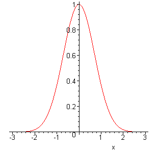
Gaussian Integral: Substitute these approximations into the integral. The integral around $t_{0}$ becomes: $I_{t_{0}} (x) \approx g (t_{0}) e^{i x S (t_{0})} \int_{- \infty}^{\infty} e^{i x \frac{1}{2} S^{''} (t_{0}) (t - t_{0})^{2}} d (t - t_{0})$ We extend the limits to $\pm \infty$ , arguing that the contribution from outside the stationary region is negligible. This is a Fresnel integral, a type of Gaussian integral, which evaluates to $2 π /∣ x S^{''} (t_{0}) ∣ e^{\pm iπ /4}$ .

The final approximation is a sum of these contributions from all stationary points. The key result is that the integral's magnitude typically scales as $1/ x$ .

2. The Method of Steepest Descent: Into the Complex Plane

The stationary phase method works beautifully for purely oscillatory exponents. But what if the exponent is complex? This is where we generalize to the method of steepest descent, also known as the saddle-point method. We consider an integral of the form:

I (x) = \int_{C} g (z) e^{x f (z)} d z

Here, $x$ is a large real parameter, $C$ is a contour in the complex plane, and $f (z)$ is an analytic function, $f (z) = u (x, y) + i v (x, y)$ .

The magnitude of the integrand is $∣ e^{x f (z)} ∣ = e^{xu (x, y)}$ , while its phase is governed by $xv (x, y)$ . The core idea is to use Cauchy's theorem, which allows us to deform the integration contour $C$ without changing the value of the integral (as long as we don't cross any singularities). We want to deform it into a new contour, $C^{'}$ , which makes the integral easier to evaluate.

What would be the ideal contour?

It should pass through a point $z_{0}$ where the magnitude $e^{xu}$ is maximal.
Along the contour, the magnitude should decrease as steeply as possible away from $z_{0}$ .
Ideally, the phase $v$ should be constant along this path to prevent oscillatory cancellations.

This seems like a lot to ask for, but the properties of analytic functions give us all three for free. This is one of the most elegant results in mathematical physics.

Lecture 6: Steepest descent

In this lecture, Professor Steven Strogatz provides a superb explanation of the method of steepest descent, unifying Laplace's method and stationary phase.

First, watch the introduction from the beginning, where he sets up the problem for a general complex exponent. Next, watch the segment from this point, where he explains the "big idea": deforming the contour to a path where the imaginary part of the exponent, v, is constant. This eliminates oscillations and reduces the problem to a Laplace-type integral. Finally, and most importantly, watch the explanation from here. This section reveals why a path of constant phase is simultaneously a path of steepest descent for the magnitude. The argument relies on the orthogonality of the gradients of u and v, a direct consequence of the Cauchy-Riemann equations which you've encountered in your complex analysis course.

Let's quickly summarize the key insight from the video. For an analytic function $f (z) = u + i v$ , the Cauchy-Riemann equations imply $\nabla u \cdot \nabla v = 0$ . This means the level curves of $u$ are orthogonal to the level curves of $v$ . The path of steepest descent for $u$ is along the direction $- \nabla u$ , which is perpendicular to the level curves of $u$ . Therefore, the path of steepest descent must lie along a level curve of $v$ . This is a remarkable connection.

The point $z_{0}$ that maximizes the integrand along the contour is a saddle point of the function $u (x, y)$ , which means $f^{'} (z_{0}) = 0$ . Near this point, the landscape of $∣ e^{x f (z)} ∣$ looks like a mountain pass. Our new contour goes up one valley, over the saddle point, and down the other valley along the path of steepest descent.

A plot of $e^{-s^2}$ along the real axis. In the steepest descent method, we deform the contour in the complex plane such that the integrand takes this Gaussian shape along the new path.

3. A Detailed Example: The Craft of Contour Deformation

Knowing the theory is one thing; applying it is another. The "craft" of this method lies in choosing the correct contour. Let's walk through a non-trivial example that illustrates the typical steps and reasoning involved. We will follow Strogatz's detailed calculation of the integral:

I (x) = \int_{0}^{1} e^{i x t^{2}} d t

Lecture 6: Steepest descent

This extended segment walks through the entire process of applying the steepest descent method to a challenging integral with finite limits.

Setup and Contour Design (Part 1): Follow the initial setup where f(z) = iz^2, leading to u = -2uv and v = u^2-v^2. Pay close attention to the logic for constructing the three-part contour (C1, C2, C3). The key is to choose paths of constant phase (v=\text{const}) and then to verify that on these paths, the magnitude part (u) has its maximum at a finite point, ensuring the integral converges and is dominated by the endpoint. Calculation and Asymptotics (Part 2): Watch how the contributions from each part of the contour are calculated. The "bridge" C2 is shown to be negligible. The path C1 gives the contribution from the stationary phase point at z=0. The path C3 gives a new contribution from the endpoint at z=1, which the standard stationary phase method would miss. This is where the power of steepest descent shines. Higher-Order Terms (Part 3): Finally, look at the "slicker approach." This demonstrates how to get not just the leading term but the next term in the asymptotic series by approximating the contour locally with its tangent line. This directly connects back to our previous lesson on building up an asymptotic series.

This example is extremely instructive. It shows that the stationary points are not just where $f^{'} (z) = 0$ , but can also include the endpoints of the original integration interval. The method of steepest descent correctly handles all these contributions by deforming the problem into the complex plane, where the contributions can be systematically evaluated as Gaussian-like integrals near the saddle points.

The general formula for the leading-order contribution from a single saddle point $z_{0}$ is:

I (x) \approx g (z_{0}) e^{x f (z_{0})} e^{i ϕ} \frac{2 π}{x ∣ f ^{''} ( z _{0} ) ∣}

where $ϕ$ is the angle of the steepest descent path through the saddle point. You can find a derivation of this compact formula in the reading below, which serves as a good summary.

The saddle-point method aka 'method of steepest descents'

This document provides a concise mathematical summary of the saddle-point method.

Read the first page of this document, from the beginning down to the final formula. This provides the general result that is derived more intuitively in the video lectures. Note the condition used to find the angle of the steepest descent path, \phi = (\pi - \theta)/2, where \theta is the phase of f''(z_0).

Conclusion

Today you have learned one of the most versatile and powerful tools for asymptotic analysis. While the details of deforming contours can be intricate, the underlying principles are elegant and deeply connected to the properties of analytic functions.

Key Takeaways:

Stationary Phase: For highly oscillatory integrals $\int g (t) e^{i x S (t)} d t$ , the dominant contributions come from points where the phase is stationary, $S^{'} (t_{0}) = 0$ . The integral typically scales as $1/ x$ .
Steepest Descent: This method generalizes stationary phase to integrals with complex exponents, $\int g (z) e^{x f (z)} d z$ . We deform the contour in the complex plane to pass through saddle points ( $f^{'} (z_{0}) = 0$ ) along paths of steepest descent.
The Magic of Analyticity: The path of steepest descent for the integrand's magnitude ( $e^{xu}$ ) is automatically a path of constant phase ( $v = const$ ). This eliminates oscillations and turns the problem into a set of Gaussian-like integrals.
The Craft: The art of the method lies in identifying all relevant saddle points (including boundary points) and constructing a valid contour that captures their contributions while ensuring other parts of the contour are negligible.

These methods are the engine for generating the asymptotic series we discussed previously. You now have a concrete procedure for taking an integral representation of a physical quantity and extracting its behavior in a limiting regime.

In our next lesson, we will apply these ideas in a slightly different context to develop the WKB approximation, a semiclassical method for solving the Schrödinger equation. We will see that the WKB ansatz, $ψ (x) \sim e^{i S (x) /ℏ}$ , casts quantum mechanics in a form that is tailor-made for an asymptotic analysis very similar to what we have learned today.

Recommended resources

1. The Principle of Stationary Phase

2. The Method of Steepest Descent: Into the Complex Plane

3. A Detailed Example: The Craft of Contour Deformation

Conclusion