Matched Asymptotic Expansions

1. Singular vs. Regular Perturbations

To begin, let's formalize the distinction between the well-behaved perturbation problems you've likely seen before and the more subtle singular ones. In a regular perturbation problem, the solution for a small, non-zero parameter $ϵ$ smoothly approaches the solution found by simply setting $ϵ=0$.

In contrast, a singular perturbation problem is one where setting $ϵ=0$ fundamentally alters the character of the problem. Most commonly, this occurs when $ϵ$ multiplies the highest-order derivative in a differential equation.

Consider an equation of the form:

If we naively set $ϵ=0$, the equation becomes first-order. A second-order ODE requires two boundary conditions to specify a unique solution, while a first-order ODE can only satisfy one. The unperturbed problem is incapable of satisfying the full set of constraints; it has lost essential information. This loss signals a singular perturbation. The region where the neglected $ϵy^{\prime \prime }$ term is actually crucial is called a boundary layer, a narrow zone of rapid change.

The following video provides an excellent introduction to this phenomenon and illustrates why a standard perturbation expansion fails.

The key idea is that the solution lives in two different worlds. In one part of the domain, the "outer region," the solution varies slowly, and the $ϵy^{\prime \prime }$ term is genuinely negligible. In another part, the "inner region" or boundary layer, the solution changes so rapidly that the second derivative $y^{\prime \prime }$ becomes enormous, making the $ϵy^{\prime \prime }$ term comparable to the others, a phenomenon known as dominant balance.

2. The Method of Matched Asymptotic Expansions

Our strategy is to find separate approximations in the inner and outer regions and then stitch them together. Let's walk through the procedure using the example from the video:

Here we've chosen the constant $a=1$ for simplicity. We anticipate the boundary layer will be at $x=0$ because the first derivative term $y^{\prime }$ tends to "push" information in the direction of increasing $x$.

Step 1: The Outer Solution

Away from the boundary layer, we assume a regular expansion works. This is the outer solution, $y_{out}(x)$. We set $ϵ=0$ in the ODE:

The general solution is $y_{out}(x)=C{e}^{-x}$. This solution cannot satisfy both boundary conditions. Since we assume the boundary layer is at $x=0$, the outer solution should be valid at $x=1$. Applying $y(1)=1$, we get $C{e}^{-1}=1$, so $C=e$.

This is our leading-order outer solution. It satisfies the boundary condition at $x=1$ but fails at $x=0$, where $y_{out}(0)=e\ne 0$.

Step 2: The Inner Solution

To resolve the physics inside the boundary layer near $x=0$, we need to "zoom in". We introduce a stretched coordinate that treats the layer's thickness (which scales with $ϵ$) as the unit of length. Let's define the inner variable $X=x/ϵ$.

Using the chain rule, derivatives with respect to $x$ become derivatives with respect to $X$:

Substituting these into the original ODE and letting $y(x)=Y(X)$ gives:

Multiplying by $ϵ$, we get the equation for the inner solution:

Notice that in the stretched coordinate $X$, the problem has become regular! The highest derivative is no longer multiplied by a small parameter. To leading order ($ϵ\to 0$), we have:

The solution is $Y_{in}(X)=A+B{e}^{-X}$. This inner solution must satisfy the boundary condition inside its domain, at $x=0$ (which is $X=0$). Applying $y(0)=0$, we get $Y_{in}(0)=A+B=0$, so $A=-B$.

This leaves one unknown constant, $B$, to be determined.

Step 3: Asymptotic Matching

The unknown constants in the inner and outer solutions are found by requiring that the two solutions smoothly join in an intermediate, "overlap" region. The simplest version of this is the Van Dyke matching principle: The outer limit of the inner solution must equal the inner limit of the outer solution.

Let's compute these limits:

• Inner limit of the outer solution: ${\lim }_{x\to 0}{y}_{out}(x)={\lim }_{x\to 0}{e}^{1-x}=e$
• Outer limit of the inner solution: ${\lim }_{X\to \infty }{Y}_{in}(X)={\lim }_{X\to \infty }B(e^{-X}-1)=-B$

Equating them gives $e=-B$, so $B=-e$. Our inner solution is now fully determined:

Rewriting in terms of the original variable $x$, we have $y_{in}(x)=e(1-e^{-x/ϵ})$.

The following resource provides a detailed walkthrough of this entire procedure, reinforcing the steps we just outlined.

Step 4: The Uniform (Composite) Solution

We now have two approximations: $y_{out}(x)$ which works well for $x\gg ϵ$, and $y_{in}(x)$ which works well for $x\sim O(ϵ)$. We can combine them into a single uniform approximation, $y_{unif}(x)$, valid across the entire domain. A common way to do this is:

Here, $y_{match}$ is the common value found during matching, which was $e$. The logic is that by adding the inner and outer solutions, we have double-counted their overlapping behavior, so we must subtract it once.

For our problem, this gives:

This single expression beautifully captures both the rapid rise in the boundary layer near $x=0$ and the slow decay in the outer region.

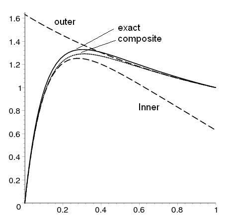
To see the complete process for this type of problem worked out, you can now watch the rest of the Kutz video.

3. A Glimpse at Higher-Order Matching

The procedure we've discussed so far gives the leading-order uniform approximation. For greater accuracy, one can carry the inner and outer expansions to higher orders in $ϵ$. This, however, requires a more sophisticated matching procedure.

The simple Van Dyke principle is the first step in a more general method developed by Lagerstrom, Kaplun, and others. The idea is to analyze the inner and outer expansions in the "intermediate" or "overlap" region in a more systematic way. A key insight, as explored in the work of Bender and Orszag, is that the matching must be performed in a region that itself shrinks as you go to higher orders.

For instance, to perform a first-order match, you might keep terms of order $x$ and $ϵ$ but neglect terms of order $x^2$, $ϵx$, and ${ϵ}^2$. This implies you are working in a region where, for example, $x\ll \sqrt{ϵ}$ but still $x\gg ϵ$. This hierarchical view of smallness is a hallmark of advanced asymptotic analysis.

The following video by Steven Strogatz provides a fascinating conceptual overview of this subtle strategy. You don't need to follow all the algebraic details, but focus on the underlying idea of how the matching region and the retained terms are defined.

This advanced technique, while algebraically intensive, allows for the systematic improvement of the approximation to any desired order in $ϵ$. It represents the full power of matched asymptotics as a rigorous analytical tool.

Conclusion

Today, we have demystified singular perturbation problems and established a robust methodology for solving them. The method of matched asymptotic expansions is a cornerstone of theoretical physics, allowing us to build accurate global solutions from simpler, locally valid pieces.

Key Takeaways:

• Singular perturbation problems typically arise when a small parameter $ϵ$ multiplies the highest derivative, causing naive expansions to fail.
• The solution involves dividing the domain into an outer region of slow variation and an inner region (boundary layer) of rapid change.
• In the inner region, a stretched coordinate (e.g., $X=x/ϵ$) restores the dominant balance and makes the problem regular.
• Unknown integration constants are determined by the asymptotic matching of the inner and outer solutions in an overlap region.
• A composite or uniform solution ($y_{unif}=y_{in}+y_{out}-y_{match}$) provides a globally valid approximation.

This powerful idea of "matching" appears in many advanced contexts. In your study of Quantum Field Theory, the Wilsonian approach to renormalization and the construction of effective field theories are conceptually similar: one constructs a "low-energy" theory (analogous to our outer solution) and determines its parameters (coupling constants) by "matching" calculations to the full, underlying theory (analogous to our inner solution) at a particular energy scale.

In our final lesson of this module, we will address another common feature of perturbation theory: the series we generate are often asymptotic, meaning they diverge. We will explore resummation techniques, which are methods for extracting precise physical information from these divergent series.