Winding Number Calculation in 1D Topological Models

Welcome back. In our previous lesson, we established the crucial distinction between geometric and topological properties. We saw that while geometric quantities like the Berry phase for a specific path are continuous and depend on local details, topological invariants are quantized integers that capture global, robust features of a system, insensitive to smooth deformations. We ended with the idea that integrating a local geometric quantity (like Berry curvature) over a closed space can yield a global topological invariant.

Today, we will make these abstract ideas concrete. We will construct and analyze the Su-Schrieffer-Heeger (SSH) model, a cornerstone of topological condensed matter physics. Our goal is to explicitly compute its characteristic topological invariant—the winding number—and understand its physical significance. This will be your first hands-on experience in how the formal methods of topology are applied to predict real physical phenomena.

The Su-Schrieffer-Heeger (SSH) Model

The SSH model is a "toy model" in the best sense of the term: it is simple enough to be solved exactly, yet rich enough to display profound topological physics. It was originally proposed to describe conduction in the polymer polyacetylene.

Imagine a one-dimensional chain of atoms. In the SSH model, these atoms are not equally spaced. Instead, they form pairs, or dimers. This results in a pattern of alternating "strong" and "weak" bonds, or equivalently, alternating hopping amplitudes for an electron moving along the chain.

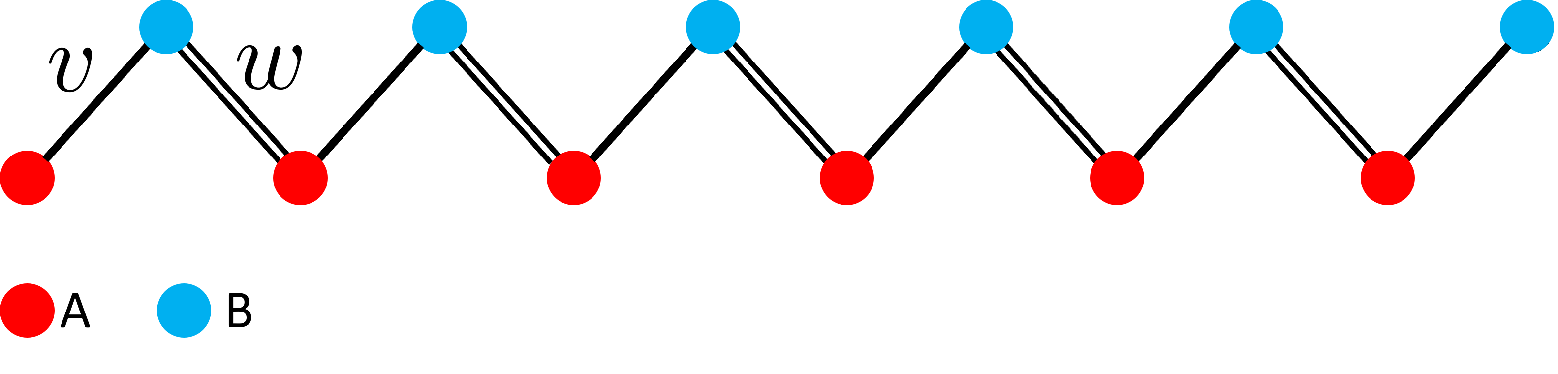
A one-dimensional chain in the SSH model. The system is composed of unit cells, each containing two distinct sites, A (red) and B (blue). The hopping amplitude for an electron within a unit cell is $v$, while the hopping between adjacent unit cells is $w$.

We can describe this system with a tight-binding Hamiltonian. Let's denote the hopping amplitude inside a unit cell (between an A and B site) as $v$ , and the hopping amplitude between unit cells as $w$ . The Hamiltonian for a chain of $N$ unit cells is:

H^= v m = 1 \sum N (∣ m, B ⟩ ⟨ m, A ∣ + h.c.) + w m = 1 \sum N - 1 (∣ m + 1, A ⟩ ⟨ m, B ∣ + h.c.)

Here, $∣ m, A ⟩$ represents an electron at the A-site of the $m$ -th unit cell, and "h.c." stands for the Hermitian conjugate.

For a long chain, it is convenient to assume periodic boundary conditions and use a Fourier transform. This allows us to describe the system in momentum space, where the Hamiltonian for each momentum $k$ becomes a simple 2×2 matrix acting on the (A, B) sublattice degree of freedom within a unit cell. This momentum-space Hamiltonian, $H^(k)$ , can be written in terms of the Pauli matrices $σ^_{x, y, z}$ :

H^(k) = d_{x} (k) σ^_{x} + d_{y} (k) σ^_{y} = d (k) \cdot σ^

where

d (k) = (d_{x} (k) d_{y} (k)) = (v + w cos (k) w sin (k))

Notice that there is no $σ^_{z}$ term. This is a consequence of a built-in property of the model called chiral symmetry, which we will explore later. The energy eigenvalues are simply $E (k) = \pm ∣ d (k) ∣$ . An energy gap exists as long as $d (k) \neq = 0$ for any $k$ . This condition is met as long as $v \neq = w$ .

Visualizing the Winding Number

This vector $d (k)$ is the key to understanding the topology of the SSH model. As the momentum $k$ sweeps across the first Brillouin zone (from $- π$ to $π$ ), the tip of the vector $d (k)$ traces out a closed loop in the $(d_{x}, d_{y})$ plane.

The winding number, $ν$ , is a topological invariant that counts how many times this loop encircles the origin $d = 0$ .

The following video provides an excellent visualization of this concept. It uses slightly different notation ( $u, v$ instead of $v, w$ , and a complex number $z$ instead of a vector $d$ ), but the idea is identical.

SYMMETRIES OF THE SSH MODEL AND END MODES

This video from Weizmann online course on topological quantum matter provides a clear, animated explanation of the winding number in the SSH model.

Please watch the segment from the winding number discussion. Focus on the two distinct cases presented: When the intracell hopping is stronger than the intercell hopping (v > w), the loop traced by the Hamiltonian vector does not enclose the origin. When the intercell hopping is stronger (w > v), the loop does enclose the origin.

As you saw, the model has two distinct insulating phases:

Trivial Phase ( $v > w$ ): The loop does not encircle the origin. The winding number $ν = 0$ . This corresponds to a chain of isolated dimers.
Topological Phase ( $w > v$ ): The loop encircles the origin once. The winding number $ν = 1$ . This corresponds to a chain where the ends of the chain are strongly coupled.

This winding number is precisely the kind of topological invariant we discussed in the last lesson. It's an integer that cannot change unless the loop passes through the origin, which corresponds to the energy gap closing ( $v = w$ )—a topological phase transition. This connects back to the homotopy concepts you've seen: we are classifying maps from the Brillouin zone (topologically a circle, $S^{1}$ ) to the space of gapped Hamiltonians (the plane minus the origin, $R^{2} ∖ {0}$ ). The relevant homotopy group is $π_{1} (R^{2} ∖ {0}) = Z$ , and our winding number $ν$ is the integer from this group.

Computing the Winding Number

Visual inspection is intuitive, but for a formal analysis, we need to compute the winding number.

Method 1: Integral of the Phase Change

The winding number can be formally defined as the total change in the angle of the vector $d (k)$ as $k$ goes from $- π$ to $π$ , divided by $2 π$ . Let $θ (k)$ be the polar angle of $d (k)$ , such that $tan θ (k) = d_{y} (k) / d_{x} (k)$ . The winding number $ν$ is then given by the integral:

ν = \frac{1}{2 π} \int_{- π}^{π} \frac{d θ ( k )}{d k} d k = \frac{θ ( π ) - θ ( - π )}{2 π}

To see how this works, consider the off-diagonal part of the Hamiltonian in matrix form:

H^(k) = (0 h^{*} (k) h (k) 0)

where $h (k) = d_{x} (k) + i d_{y} (k) = v + w e^{ik}$ . The winding number can be written as an integral over the phase of this complex function:

ν = \frac{1}{2 π i} \int_{- π}^{π} \frac{1}{h ( k )} \frac{d h ( k )}{d k} d k = \frac{1}{2 π i} \int_{- π}^{π} \frac{d}{d k} (lo g h (k)) d k

This integral simply counts the winding of the complex number $h (k)$ around the origin in the complex plane, which is exactly what we visualized.

Method 2: A Shortcut with Complex Analysis

Given your mathematics minor, you might appreciate a more elegant method using complex analysis. The integral over the Brillouin zone can be transformed into a contour integral over the unit circle in the complex plane. Let's make the substitution $z = e^{ik}$ . Then $d k = d z / (i z)$ , and our function becomes $h (k) \to f (z) = v + w z$ .

The winding number integral transforms into:

ν = \frac{1}{2 π i} \oint_{∣ z ∣ = 1} \frac{f ^{'} ( z )}{f ( z )} d z

From the Argument Principle in complex analysis, you'll recall that this integral counts the number of zeros ( $Z$ ) minus the number of poles ( $P$ ) of the function $f (z)$ inside the contour (the unit circle).

Our function is $f (z) = v + w z$ .

Poles: $f (z)$ has no poles inside the unit circle, so $P = 0$ .
Zeros: $f (z)$ has a single zero at $z_{0} = - v / w$ .

Now we check if this zero is inside the contour:

Trivial Case ( $v > w$ ): Here, $∣ z_{0} ∣ = v / w > 1$ . The zero is outside the unit circle. Thus, $Z = 0$ . The winding number is $ν = Z - P = 0 - 0 = 0$ .
Topological Case ( $w > v$ ): Here, $∣ z_{0} ∣ = v / w < 1$ . The zero is inside the unit circle. Thus, $Z = 1$ . The winding number is $ν = Z - P = 1 - 0 = 1$ .

This confirms our visual intuition and the results of the phase integral with remarkable efficiency. The topological distinction between the two phases is encoded in the location of a zero in the complex plane.

To solidify these concepts, please study the following resources.

[PDF] A Short Course on Topological Insulators

This chapter from the textbook by Asbóth, Oroszlányi, and Pályi provides a rigorous yet clear derivation of the winding number for the SSH model.

Please read the sections Winding Number of the SSH Model and the subsequent short paragraph ending in ν = 1. This will walk you through the definition of the winding number for the \mathbf{d}(k) vector and explicitly state the result for the two phases.

[PDF] Bulk-Edge Correspondence in the 1D SSH Model

This paper provides a concise derivation of the winding number using the complex analysis approach we just discussed.

Read section Winding Number calculation. Also, review the short section Topological Phase Transition in the Standard SSH Model. This will reinforce the calculation and its physical interpretation. Note: The paper's convention for h(k) may differ slightly, but the method and final conclusion are the same.

From Winding Number to Physical Consequences

Why is this integer so important? The winding number is not just a mathematical curiosity; it has profound physical consequences, a principle known as the bulk-boundary correspondence. The SSH model provides the simplest and clearest example of this principle:

A system with a trivial bulk topological invariant ( $ν = 0$ ) will have conventional, gapped boundaries.
A system with a non-trivial bulk topological invariant ( $ν = 1$ ) is guaranteed to host special, protected states at its boundaries.

For the SSH model, if you take a finite chain in the topological phase ( $w > v$ ), you will find a single state localized at each end of the chain with an energy of exactly zero, right in the middle of the bulk energy gap. These "zero-energy edge modes" are topologically protected: you cannot get rid of them by any smooth change to the Hamiltonian (like adding disorder) that preserves the gap and the underlying symmetries. The existence of these robust edge states is directly predicted by the non-zero winding number of the bulk.

The following video discusses this connection and the physical origin of the two phases in polyacetylene.

TMS21 Lecture 2. Jennifer Cano. Introduction to Topological Insulators, part 1

This lecture by Prof. Jennifer Cano provides a clear physical picture of the SSH model and its bulk-edge correspondence.

First, watch the explanation of the model from the SSH example. This connects the two phases to different bond dimerizations and explicitly links the winding number to the polarization and Berry phase. Then, watch the segment on the bulk-edge correspondence, which shows how a boundary between the two phases traps a zero-energy state.

Conclusion

In this lesson, we have moved from the abstract world of topology to a concrete physical model. We have seen how a simple 1D system can be characterized by a topological invariant, the winding number, which distinguishes between a trivial and a topological phase.

Key Takeaways:

The SSH model describes a 1D dimerized chain with two insulating phases, determined by the relative strength of intra-cell ( $v$ ) and inter-cell ( $w$ ) hopping.
The momentum-space Hamiltonian $H^(k)$ can be mapped to a vector $d (k)$ that traces a loop as $k$ spans the Brillouin zone.
The winding number $ν$ counts how many times this loop encircles the origin. It is the topological invariant for this model.
We can compute the winding number either by integrating the change in phase of the Hamiltonian vector or by using the argument principle from complex analysis.
The winding number is $ν = 0$ for the trivial phase ( $v > w$ ) and $ν = 1$ for the topological phase ( $w > v$ ).
The bulk-boundary correspondence guarantees that the non-trivial bulk topology ( $ν = 1$ ) gives rise to robust, zero-energy states localized at the edges of a finite system.

You now have the tools to analyze a topological model and compute its defining invariant. In our next lesson, we will extend these ideas to two dimensions. We will revisit the Berry curvature from earlier lessons and see how integrating it over the 2D Brillouin zone yields another famous topological invariant, the Chern number, which is central to understanding the integer quantum Hall effect.

Recommended resources