Chern Number Calculation: Berry Curvature Integration

From Berry Curvature to a Topological Invariant

Let's begin by solidifying the link between the Berry phase, which you know is path-dependent, and a truly topological quantity. The key concepts are the Berry connection (or potential), ${\mathbf{A}}_n(\mathbf{k})$, and the Berry curvature, ${\Omega }_n(\mathbf{k})$, for a given energy band $n$.

As you've seen, these quantities are formally analogous to the vector potential and magnetic field in electromagnetism. The Berry connection is defined from the cell-periodic part of the Bloch wavefunctions, $|u_{n\mathbf{k}}⟩$:

The Berry curvature is its "curl" in momentum space:

Just as the magnetic flux is the integral of the magnetic field, the Berry phase ${\gamma }_n$ acquired along a closed loop $C$ in the Brillouin zone is the "flux" of the Berry curvature through the surface $S$ enclosed by that loop. This is a direct application of Stokes' theorem.

The following video provides an excellent summary of these relationships, culminating in the definition of the Chern number.

The crucial insight here is that while the Brillouin zone of a 1D crystal is a circle ($S^1$), the BZ of a 2D crystal is a torus ($T^2=S^1\times S^1$). A torus is a closed surface with no boundary. Therefore, integrating the Berry curvature over the entire 2D Brillouin zone is an integral over a closed manifold.

A fundamental result, known as the Chern theorem, states that such an integral is always quantized. Specifically, the integral of the Berry curvature of an isolated band $n$ over a closed 2D manifold (like the BZ) must be an integer multiple of $2\pi$. This integer is the first Chern number, $C_n$.

This integer $C_n$ is the topological invariant for 2D systems, playing the same role as the winding number $\nu$ in 1D. A band with $C_n=0$ is topologically trivial, while a band with $C_n\ne 0$ is non-trivial.

For a more formal treatment of this quantization, the following reading provides a proof of the Chern theorem. Given your mathematics minor, you should find the argument illuminating.

The Haldane Model: A Chern Insulator

To make this concrete, we need a 2D toy model, analogous to how the SSH model served us in 1D. The canonical example is the Haldane model, proposed by F. Duncan Haldane in 1988. It was a theoretical breakthrough, showing that a system could exhibit a quantum Hall effect without any net external magnetic field—a "Chern insulator."

The model starts with graphene, a single sheet of carbon atoms arranged in a honeycomb lattice. Graphene's Hamiltonian has two energy bands that touch at two specific points in the Brillouin zone, the Dirac points K and K'. Because of time-reversal and inversion symmetries, the Berry curvature of a given band has opposite signs around the K and K' points. When integrated over the entire BZ, these contributions exactly cancel, resulting in a Chern number of zero for each band.

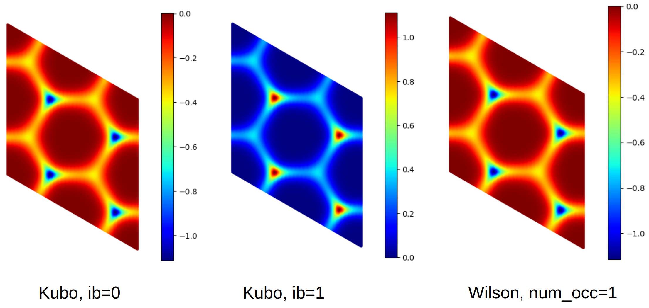
Haldane's brilliant idea was to add a term to the Hamiltonian that breaks time-reversal symmetry but preserves the translational symmetry of the lattice and, crucially, produces no net magnetic flux through the unit cell. This is achieved by introducing complex hopping amplitudes between next-nearest-neighbor atoms.

This new term has two effects:

1. It opens an energy gap at the K and K' points, turning the semimetal into an insulator.
2. It modifies the Berry curvature landscape such that the contributions from K and K' no longer cancel.

The result is a phase with a non-zero Chern number. The following video introduces the model and its properties.

Computing the Chern Number

Now for the main task: how do we actually compute the Chern number for a model like Haldane's? There are two primary strategies.

1. The Direct (Numerical) Method

The definition of the Chern number is an integral. In practice, this integral is performed numerically. The standard method is to:

1. Discretize the 2D Brillouin zone into a fine grid of $N\times N$ points.
2. For each small plaquette in this grid, compute the Berry phase accumulated around its four corners. This gives a local, discrete version of the Berry curvature.
3. Sum the phases from all plaquettes over the entire BZ.

Due to the Chern theorem, this sum (divided by $2\pi$) must converge to an integer as the grid becomes finer. This method is computationally straightforward and is how Chern numbers are typically calculated in numerical simulations.

2. The Physicist's Shortcut: Tracking Gap Closings

A more elegant and physically insightful method avoids direct integration. Since the Chern number is a topological invariant, it cannot change as long as the energy gap remains open. It can only change when the system undergoes a topological phase transition, which occurs precisely when the gap closes.

The strategy is as follows:

1. Start in a trivial limit of the model where the Chern number is obviously zero (e.g., when the Haldane term is turned off, or a large mass term dominates).
2. Vary a parameter of the model (e.g., the mass term $m$) and find the critical values where the gap closes. In the Haldane model, these closings happen at the K and K' points.
3. Near each gap-closing point, the low-energy Hamiltonian can be approximated by a massive 2D Dirac Hamiltonian. A key result is that each such massive Dirac point contributes exactly $\pm 1/2$ to the total Chern number. The sign depends on the sign of the effective mass term.
4. By tracking the sign of the mass term as we cross each critical point, we can determine the change $\Delta C$ in the Chern number. Summing these changes allows us to map out the entire topological phase diagram.

This powerful technique reduces the problem of a 2D integral to analyzing the behavior at a few discrete points in parameter space.

With the knowledge that each gap closing at a Dirac point changes $C$ by $\pm 1$, we can now construct the phase diagram of the Haldane model simply by finding where the gaps close at K and K'. The video you watched earlier and the following reading both execute this strategy perfectly.

To reinforce this, you can read through a similar derivation in the ETH Zurich notes, which applies the same logic to the Haldane model. Reading this will solidify your understanding of the technique. You can find this in Section 4.3 of the "Chern insulators" document (resource LINK).

Conclusion

In this lesson, we have made the leap from one to two dimensions in the study of topological matter. We have defined the Chern number, a robust integer invariant that classifies 2D energy bands, and shown how it emerges from integrating the Berry curvature over the Brillouin zone.

Key Takeaways:

• The Chern number $C_n=\frac{1}{2\pi }{\oint }_{\text{BZ}}{\Omega }_n{d}^{2}k$ is the topological invariant that characterizes the $n$-th band of a 2D insulator. It must be an integer.
• A non-zero Chern number requires broken time-reversal symmetry.
• The Haldane model on a honeycomb lattice is the canonical example of a Chern insulator—a system with non-zero Chern numbers for its bands even with zero net magnetic field.
• The Chern number can be computed directly by numerical integration of the Berry curvature over a discretized Brillouin zone.
• A more physical method is to track gap closings. By starting in a trivial phase ($C=0$) and identifying how the low-energy Dirac mass terms change sign at topological phase transitions, one can deduce the Chern number in all phases.

You have now added a second, fundamental topological invariant to your toolkit. In our next lesson, we will complete this part of our journey by exploring the physical consequences of these invariants. We will see how, through the bulk-boundary correspondence, a non-zero Chern number in the bulk mandates the existence of chiral, conducting edge states—the hallmark of the integer quantum Hall effect.