Topological Classification of Physical Systems

Welcome to our second lesson on the mathematical toolkit for theoretical physics. In our previous session, we explored how group theory provides a powerful framework for classifying quantum states and particles based on their symmetries. We saw that the structure of a system's symmetry group dictates the very nature of its constituents.

Today, we shift our focus from symmetry to another profound organizational principle: topology. While group theory is concerned with what remains invariant under specific transformations like rotations or translations, topology deals with properties that are robust against any continuous deformation—stretching, twisting, and bending, but not tearing or gluing. This lesson will introduce you to the key topological concepts of manifolds and homotopy, and demonstrate how they provide a surprisingly powerful method for classifying physical systems, particularly the exotic defects that can emerge in condensed matter. By the end of this lesson, you will be able to use homotopy groups to predict the existence and stability of topological defects in a given physical system.

1. The Arenas of Physics: Topological Manifolds

Most of modern physics takes place on mathematical spaces called manifolds. Intuitively, a manifold is a space that, on a small enough scale, looks like our familiar Euclidean space, $R^{d}$ . For example, the surface of the Earth is a 2-dimensional manifold; while it is globally a sphere, any small patch of it looks approximately like a flat plane. This "local flatness" is the key property that allows us to do calculus and define concepts like velocity and acceleration.

To formalize this, physicists and mathematicians use the language of charts and atlases. A chart is a map from a small open patch of the manifold to an open set in $R^{d}$ . An atlas is a collection of charts that covers the entire manifold. This is precisely how a real-world atlas works: each page is a chart (a flat map of a small region), and the whole book covers the globe.

Topological manifolds and manifold bundles- Lec 06 - Frederic Schuller

Professor Frederic Schuller provides a clear and physically-motivated introduction to topological manifolds in this lecture.

First, watch the section from the definition of a topological manifold. This will formalize the idea of a space that "locally looks like RD". Then, to connect this abstract definition to the familiar language of physics, watch the segment on charts and atlases. Pay close attention to the idea that the coordinates of a point are not intrinsic to the point itself, but depend on the chart you use to describe it. This is the formal basis for the "coordinate independence" that is so crucial in theories like General Relativity.

The key takeaway is that manifolds provide the stage for our physical theories, and their global topological structure can have profound physical consequences, even if they look the same locally. The sphere S², the torus T², and the real projective plane RP² are all 2-dimensional manifolds, but as we will see, their different global topologies lead to vastly different physical possibilities.

2. Classifying Holes: Homotopy and the Fundamental Group

How can we mathematically distinguish between a sphere and a torus? We can't just "look" at them. Topology provides a rigorous way to do this by classifying their "holes." The tool for this is homotopy theory.

Homotopy is the study of continuous deformations of maps. For our purposes, we are interested in maps that represent loops in a space. Consider a loop drawn on a surface. Can this loop be continuously shrunk down to a single point without leaving the surface?

On a flat plane ( $R^{2}$ ) or the surface of a sphere (S²), any loop can be shrunk to a point. We say these spaces are simply connected.
On the surface of a doughnut (a torus, T²), a loop that goes around the hole cannot be shrunk to a point. Neither can a loop that goes through the hole.
On a plane with a single point removed ( $R^{2} ∖ {p}$ ), which is topologically like a cylinder or an annulus, a loop that encircles the missing point cannot be shrunk.

The fundamental group, denoted $π_{1} (M)$ , formalizes this idea. It is the group formed by all the equivalence classes of loops on a manifold $M$ , where two loops are considered equivalent if one can be continuously deformed into the other. The "multiplication" operation in this group is simply concatenating two loops: first traversing one, then the other.

The fundamental group essentially counts the number of distinct, non-deformable types of 1-dimensional "holes" in a space.

Topology and geometry for physicists

This document by Emanuel Malek provides a concise, physicist-friendly introduction to homotopy groups.

Please read the sections up to loop products and then from homotopy of loops to the group definition. This introduces the core concepts of loops, their products, and how the set of homotopy classes of loops forms the fundamental group, \pi_1. Finally, read the section on path-connectedness, which explains the important result that for the spaces we care about in physics, the choice of base point for the loops doesn't matter.

Here are some of the most important fundamental groups for physics:

Euclidean Space: $π_{1} (R^{d}) = {0}$ . The trivial group, with only one element (the identity). All loops are contractible.
The Circle (S¹): $π_{1} (S^{1}) = Z$ . The group of integers under addition. Each integer corresponds to a "winding number"—how many times a loop wraps around the circle (positive for one direction, negative for the other).

Loops on a circle S¹ are classified by an integer winding number. A loop that goes around once (+1) cannot be continuously deformed into a loop that goes around twice (+2) or one that doesn't go around at all (0, the identity). These distinct classes form the elements of the fundamental group $\pi_1(S^1) = \mathbb{Z}$.

Higher-dimensional Spheres (Sⁿ): For $n \geq 2$ , $π_{1} (S^{n}) = {0}$ . This is a crucial, perhaps counter-intuitive, result. Any loop on the surface of a 3D sphere (or higher) can be slid off and shrunk to a point. The hole is in the "middle," but a 1D loop can't detect it.
The Torus (T²): $π_{1} (T^{2}) = Z \oplus Z = Z^{2}$ . An element of this group is a pair of integers $(n, m)$ , where $n$ is the number of times the loop winds around the "short" way and $m$ is the number of times it winds around the "long" way.

3. Higher-Dimensional Holes: Higher Homotopy Groups

The fundamental group $π_{1}$ detects 1-dimensional loops that can't be shrunk. What about higher-dimensional holes? For instance, the hollow interior of a sphere S² isn't detected by $π_{1} (S^{2})$ . To detect this, we need to see if a 2-dimensional sphere wrapped around our space can be shrunk to a point.

This leads to the idea of higher homotopy groups, $π_{n} (M)$ . $π_{n} (M)$ is the group of homotopy classes of maps from an n-sphere, Sⁿ, into the manifold $M$ . Intuitively:

$π_{1} (M)$ classifies non-shrinkable loops (S¹ maps).
$π_{2} (M)$ classifies non-shrinkable wrapped spheres (S² maps).
$π_{3} (M)$ classifies non-shrinkable wrapped 3-spheres (S³ maps), and so on.

A key result is that for $n \geq 2$ , all higher homotopy groups $π_{n}$ are abelian (commutative). Calculating these groups is a major focus of algebraic topology. For our purposes, we can rely on tabulated results.

Homotopy in statistical physics

This review by Ralph Kenna provides a clear introduction to higher homotopy groups and includes a very useful table.

Read the section "The higher homotopy groups". Focus on the intuition of using n-loops to detect higher-dimensional holes. Then, study Table 1, which lists the homotopy groups of the n-sphere, \pi_m(S^n). Notice that \pi_n(S^n) = \mathbb{Z} and \pi_1(S^n)=\{0\} for n \geq 2.

4. Application: Classifying Topological Defects

Now we arrive at the central application for this lesson. In many physical systems, particularly in your field of condensed matter, a system can develop a background "texture" described by an order parameter. This order parameter is a field that takes values in some manifold $M$ , called the order parameter space.

A topological defect is a point, line, or surface where this order parameter field is singular or ill-defined. The stability of these defects—the fact that they cannot be smoothed out by small, local perturbations—is guaranteed by the topology of the order parameter space $M$ .

The classification scheme is remarkably elegant:
An m-dimensional defect in a d-dimensional physical space is classified by the homotopy group $π_{d - m - 1} (M)$ .

If this group is trivial ( ${0}$ ), no stable defects of that type can exist. If the group is non-trivial, its elements classify the different types of defects.

Let's see this in action with some examples you'll encounter in your studies.

Homotopy in statistical physics

The Kenna review clearly states and explains this classification scheme.

Please read the section on defect classification. This text explicitly presents the key formula and the naming convention for different defect types (domain walls, vortices, monopoles).

Example 1: Vortices in a 2D Superfluid or XY Magnet

Physical Space: A 2D plane, so $d = 2$ .
Order Parameter Space: The order parameter is a complex number with fixed magnitude but variable phase, $ψ = ∣ ψ ∣ e^{i θ}$ . The phase $θ$ lives on a circle, so the order parameter space is $M = S^{1}$ .
Defects: We look for point defects ( $m = 0$ ). The relevant group is $π_{d - m - 1} (M) = π_{2 - 0 - 1} (S^{1}) = π_{1} (S^{1}) = Z$ .
Physical Interpretation: Stable point defects exist and are classified by an integer. This integer is the winding number of the phase field $θ$ as we trace a loop in the physical space around the defect core. We call these defects vortices. A vortex with charge +1 cannot be continuously unwound into a state with no vortex (charge 0).

Example 2: Defects in a 3D Ferromagnet

Physical Space: 3D space, so $d = 3$ .
Order Parameter Space: The order parameter is the magnetization vector $m$ , which has a fixed magnitude but can point in any direction. The space of all possible directions is a 2-sphere, so $M = S^{2}$ .
Line Defects (Vortices): $m = 1$ . The group is $π_{3 - 1 - 1} (S^{2}) = π_{1} (S^{2}) = {0}$ .
- Physical Interpretation: Because the fundamental group of the 2-sphere is trivial, stable line defects do not exist in a 3D ferromagnet. Any vortex line can "slip off" the sphere and unwind.
Point Defects (Monopoles): $m = 0$ . The group is $π_{3 - 0 - 1} (S^{2}) = π_{2} (S^{2}) = Z$ .
- Physical Interpretation: Stable point defects exist and are classified by an integer. This corresponds to how many times the magnetization vector field "wraps around" a sphere in physical space enclosing the defect. These are topological monopoles.

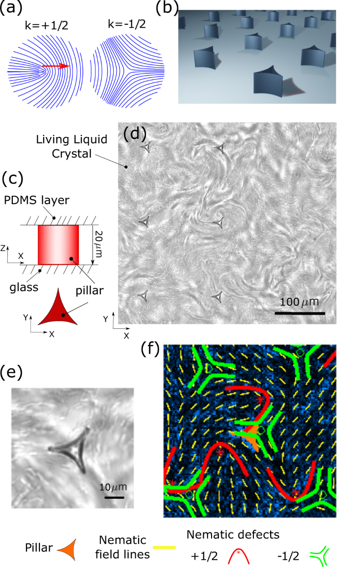
Example 3: Defects in a Nematic Liquid Crystal
Your background in soft matter makes this a particularly interesting case. In a nematic liquid crystal, the molecules align along a particular axis, but there is no preferred direction along that axis (i.e., head and tail are equivalent).

Physical Space: 3D space, $d = 3$ .
Order Parameter Space: The order parameter is a line through the origin, not a vector. This space is the 2-sphere with antipodal points identified, $M = S^{2} / Z_{2}$ , which is called the real projective plane, $R P^{2}$ . The topology of $R P^{2}$ is different from $S^{2}$ .
Line Defects (Disclinations): $m = 1$ . The relevant group is $π_{3 - 1 - 1} (R P^{2}) = π_{1} (R P^{2}) = Z_{2}$ . This is the group with two elements, ${0, 1}$ , where $1 + 1 = 0$ .
- Physical Interpretation: There is exactly one type of stable line defect. A loop in the order parameter space corresponding to this defect cannot be shrunk to a point. However, traversing it twice is shrinkable. This means two such defects can annihilate each other. This is fundamentally different from the integer-charged vortices in the XY model.
Point Defects: $m = 0$ . The group is $π_{3 - 0 - 1} (R P^{2}) = π_{2} (R P^{2}) = Z$ .
- Physical Interpretation: Integer-charged point defects, similar to the monopoles in the ferromagnet, can exist.

Defects in a nematic liquid crystal. Panel (a) shows the director field lines for +1/2 and -1/2 defects, corresponding to the non-trivial element of $\pi_1(RP^2)$. Panel (d) shows an experimental image of such defects created by pillars in a thin film. The ability to classify these stable structures is a direct consequence of the non-trivial topology of the order parameter space.

Conclusion

In this lesson, we have added a second major pillar to our theoretical toolkit. Where group theory classifies states by their transformation properties under symmetries, topology classifies systems and phases of matter by their robust, global features.

Manifolds provide the mathematical stage on which physical theories are set.
Homotopy groups ( $π_{n}$ ) are topological invariants that rigorously classify the "holes" or non-shrinkable structures within a manifold.
This mathematical framework finds a direct physical application in the classification of topological defects. By identifying the system's order parameter space $M$ , we can use its homotopy groups to predict the existence, stability, and types of defects that can occur.
The formula $π_{d - m - 1} (M)$ is a powerful predictive tool, connecting the dimensionality of space and the defect to the topology of the order parameter.

This approach has become central to modern condensed matter physics, leading to the discovery of topological insulators, the quantum Hall effect, and other exotic phases of matter where topology, not symmetry, is the guiding principle.

In our next lesson, we will step back from these high-level classification schemes and focus on a more workhorse tool: vector calculus. We will specifically tackle line and surface integrals, developing the calculational fluency needed to compute physical quantities defined on the manifolds we have discussed today.

Recommended resources

1. The Arenas of Physics: Topological Manifolds

2. Classifying Holes: Homotopy and the Fundamental Group

3. Higher-Dimensional Holes: Higher Homotopy Groups

4. Application: Classifying Topological Defects

Conclusion