Vector Calculus: Line and Surface Integrals

1. Line Integrals: Accumulating a Field Along a Path

The fundamental idea of a line integral is to sum up the effect of a vector field along a curve. The most intuitive physical motivation for this is the concept of work.

Imagine pushing an object through a region where a force field $\vec{F}$ (like wind or a magnetic force) is present. As you move the object along a path $C$, the work done on it by the field depends on two things at every point: the strength of the force, and how much that force is aligned with your direction of motion. A force perpendicular to your path does no work, while a force that opposes you does negative work. The total work is the sum of these contributions from every infinitesimal step along the path.

This physical picture leads directly to the mathematical definition of a line integral of a vector field.

As the video explains, we can formalize this in two key ways:

1. The Conceptual Definition: The line integral of a vector field $\vec{F}$ along a curve $C$ is written as
   ${\int }_C\vec{F}\cdot \hat{T}ds$
   Here, at each point on the curve, we take the dot product of the vector field $\vec{F}$ with the unit tangent vector $\hat{T}$ (the direction of the curve). This projects $\vec{F}$ onto the path. We then multiply by the infinitesimal arc length $ds$ and "add up" (integrate) these contributions along the entire curve $C$.

2. The Computational Formula: To actually calculate this, we parameterize the curve $C$ by a vector function $\vec{r}(t)$ for $t$ from $a$ to $b$. This turns the line integral into a standard one-dimensional integral with respect to the parameter $t$:
   ${\int }_C\vec{F}\cdot d\vec{r}={\int }_a^b\vec{F}(\vec{r}(t))\cdot \frac{d\vec{r}}{dt}dt$
   Let's break down this powerful formula, which is the workhorse for all line integral calculations:

   • $\vec{F}(\vec{r}(t))$: We evaluate the vector field only on the points of the curve.
   • $\frac{d\vec{r}}{dt}$: This is the velocity vector, which is tangent to the curve. It combines both the direction ($\hat{T}$) and the rate of traversal ($ds/dt$).
   • $\vec{F}\cdot \frac{d\vec{r}}{dt}$: This dot product gives us a scalar function of $t$.
   • ${\int }_a^b\dots dt$: We integrate this scalar function over the range of the parameter $t$.

The notation ${\int }_C\vec{F}\cdot d\vec{r}$ is common in physics. It treats the infinitesimal displacement along the curve, $d\vec{r}=dx\hat{ı}+dy\hat{ȷ}+dz\hat{k}$, as a vector. Thinking of the integral as summing up the dot products $\vec{F}\cdot d\vec{r}$ often aligns more closely with a physicist's picture of summing up infinitesimal contributions.

Let's see this in action.

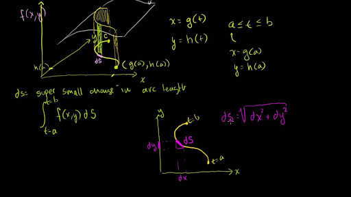
The fact that the integral's value can depend on the path taken is a crucial feature. This leads us to a special, and very important, class of vector fields.

2. Path-Independence and Conservative Fields

In the example above, the line integral depended on the path. However, for some special vector fields, the value of the line integral between two points is the same regardless of the path taken. These are called conservative vector fields.

Your physics background has already made you intimately familiar with these: the static electric field and the gravitational field are prime examples. The work done by gravity moving an object from height $h_1$ to $h_2$ is $mg(h_1-h_2)$, regardless of the rollercoaster track it took to get there. This is the essence of path-independence.

There are several equivalent properties that define a conservative field $\vec{F}$:

1. The line integral ${\int }_A^B\vec{F}\cdot d\vec{r}$ is path-independent.
2. The line integral around any closed loop is zero: $\oint \vec{F}\cdot d\vec{r}=0$.
3. The field is the gradient of some scalar function $\varphi$, called the scalar potential: $\vec{F}=\nabla \varphi$. (For forces, we often use $\vec{F}=-\nabla V$, where $V$ is the potential energy).
4. The curl of the field is zero: $\nabla \times \vec{F}=\vec{0}$.

This last property, $\nabla \times \vec{F}=\vec{0}$, is often the easiest way to test if a field is conservative. If it is, we can use property 3 to simplify calculations immensely via the Fundamental Theorem for Line Integrals:

If you can find the potential function $\varphi$, evaluating the line integral reduces to simply evaluating $\varphi$ at the start and end points and taking the difference, completely bypassing the need for parameterization.

Beyond calculating work, line integrals have other important physical interpretations. If $\vec{v}$ is the velocity field of a fluid, then ${\oint }_C\vec{v}\cdot d\vec{r}$ is the circulation around the closed loop $C$. It measures the net tendency of the fluid to rotate or swirl along the path. A non-zero circulation indicates the presence of "swirliness" (vorticity) inside the loop.

3. Surface Integrals: Accumulating a Field Through a Surface

Just as line integrals sum a field's component along a curve, surface integrals sum a field's component through a surface. The classic physical motivation is flux, which measures the rate of flow of something across a surface.

Imagine a stream with water flowing with velocity $\vec{v}$. If you place a net in the water, the amount of water passing through the net per unit time (the flux) depends on the velocity of the water and the orientation of the net. If the net is face-on to the flow, you get maximum flux. If it's edge-on, you get zero flux.

This introduces the key elements for a surface integral: the vector field $\vec{F}$ and the vector surface element $d\vec{S}$. The vector $d\vec{S}$ has a magnitude equal to the infinitesimal area $dS$ and a direction given by the unit normal vector $\hat{n}$ to the surface: $d\vec{S}=\hat{n}dS$.

The flux is then the integral of the component of $\vec{F}$ normal to the surface, summed over the whole surface $S$:
$\text{Flux}={\iint }_S\vec{F}\cdot \hat{n}dS={\iint }_S\vec{F}\cdot d\vec{S}$

How do we compute this? Analogous to line integrals, we parameterize the surface using two parameters, $u$ and $v$, with a position vector $\vec{r}(u,v)$.

This gives us the computational formula for the surface integral:
${\iint }_S\vec{F}\cdot d\vec{S}={\iint }_D\vec{F}(\vec{r}(u,v))\cdot \left(\frac{\partial \vec{r}}{\partial u}\times \frac{\partial \vec{r}}{\partial v}\right)dudv$
where $D$ is the domain in the $uv$-plane that corresponds to the surface $S$. The steps are:

1. Parameterize the surface $S$ with $\vec{r}(u,v)$.
2. Calculate the tangent vectors $\frac{\partial \vec{r}}{\partial u}$ and $\frac{\partial \vec{r}}{\partial v}$.
3. Compute the normal vector by taking their cross product. Be mindful of the direction (outward/inward) required by the problem.
4. Evaluate the field $\vec{F}$ on the surface, $\vec{F}(\vec{r}(u,v))$.
5. Compute the dot product and integrate the resulting scalar function of $u$ and $v$ over the parameter domain $D$.

Let's look at a straightforward example.

4. The Integral Theorems: A Unified Picture

The tools of line and surface integrals are tied together by three of the most important theorems in vector calculus, which are pillars of theoretical physics (especially electromagnetism and fluid dynamics). We won't derive them here, but it's crucial to know what they say. They relate an integral over a region to an integral over its boundary.

• Green's Theorem (2D): Relates the circulation of a field $\vec{F}$ around a closed curve $C$ in the plane to the integral of the curl's z-component over the area $A$ enclosed by the curve.
  ${\oint }_C\vec{F}\cdot d\vec{r}={\iint }_A(\nabla \times \vec{F}{)}_{z}dA$

• Stokes' Theorem (3D): Generalizes Green's theorem. It relates the circulation of $\vec{F}$ around a closed loop $C$ to the flux of the curl, $\nabla \times \vec{F}$, through any surface $S$ bounded by that loop.
  ${\oint }_C\vec{F}\cdot d\vec{r}={\iint }_S(\nabla \times \vec{F})\cdot d\vec{S}$

• Divergence (Gauss's) Theorem (3D): Relates the flux of $\vec{F}$ out of a closed surface $S$ to the integral of the divergence, $\nabla \cdot \vec{F}$, over the volume $V$ enclosed by the surface.
  $\iint \vec{F}\cdot d\vec{S}={\iiint }_V(\nabla \cdot \vec{F})dV$

These theorems form the foundation of Maxwell's equations in their integral form and allow physicists to move between microscopic (differential) and macroscopic (integral) descriptions of a system. For example, the Divergence Theorem says that the total flux coming out of a box is equal to the sum of all the little sources (divergence) inside the box.

Conclusion

In this lesson, we have built up the operational machinery of vector calculus. We focused on gaining the fluency to translate physical questions into calculable line and surface integrals.

• Line integrals ($\int \vec{F}\cdot d\vec{r}$) sum the tangential component of a vector field along a path. They are used to calculate quantities like work and circulation.
• Surface integrals ($\iint \vec{F}\cdot d\vec{S}$) sum the normal component of a vector field through a surface. They are used to calculate flux.
• The key to computation in both cases is parameterization: reducing the problem to a standard single or double integral over the parameters.
• A special class of conservative fields ($\nabla \times \vec{F}=\vec{0}$) have path-independent line integrals, which can be evaluated simply using a scalar potential $\varphi$.
• Finally, the great integral theorems of Green, Stokes, and Gauss unite these concepts, relating the behavior of a field on a boundary to the behavior of its derivatives (curl or divergence) in the interior.

You now have the tools to compute quantities defined on the curves and surfaces that exist within the manifolds we discussed in the last lesson. In our next session, we will add another powerful computational tool to our arsenal: complex analysis. We'll see how contour integration provides a surprisingly elegant and powerful method for solving a wide variety of real-valued integrals that appear frequently in physics.