Neural Network Training: Forward Pass, Backward Pass, and Optimization

The Training Loop: A High-Level View

Before we break it down, let's get a quick, animated overview of the entire process. The following video sketch from HuggingFace provides a perfect conceptual map of what we're about to dissect.

As the video showed, the process is a cycle of prediction, error calculation, and refinement. Now, let's name the parts of that cycle and examine them in detail.

The three core steps are:

1. Forward Pass: The network makes a prediction and we calculate how "wrong" it is.
2. Backward Pass: We calculate the contribution of each model parameter to this error.
3. Optimizer Step: We update the parameters to reduce the error for the next time.

This diagram shows how data and error flow through the network during these passes.

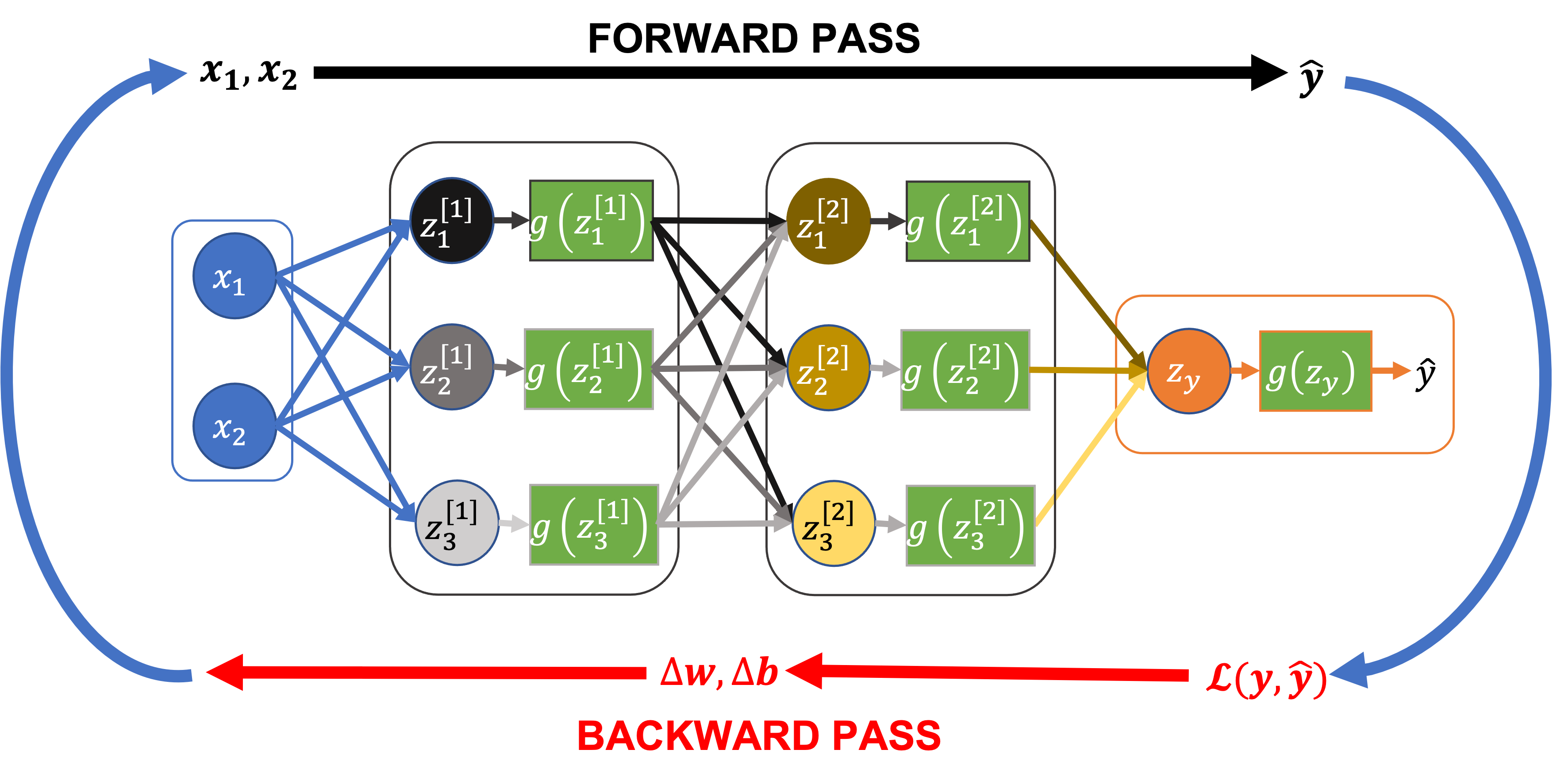
Step 1: The Forward Pass (Prediction & Loss)

The forward pass is the most intuitive part. It's where the network does what it's designed to do: make a prediction.

1. Input Propagation: You feed a batch of data (e.g., images, text) into the input layer of the network.
2. Computation: The data flows "forward" through the network's layers. At each layer, it undergoes mathematical operations (which we'll cover in the next lesson) and is transformed.
3. Prediction: The final layer produces an output, which is the model's prediction (ŷ in the diagram).
4. Loss Calculation: This prediction is compared to the ground truth (the correct answer, y) using a loss function. The loss function (e.g., Mean Squared Error) computes a single number that quantifies the model's error. A high loss means a bad prediction; a low loss means a good one.

The entire goal of training is to minimize this loss value.

Step 2: The Backward Pass (Calculating Gradients)

Once we have the loss, we need to figure out how to adjust our model's parameters (its internal weights and biases) to reduce it. This is the job of the backward pass, also known as backpropagation.

This is perhaps the least intuitive but most crucial step. You can think of it as a system for assigning "blame" for the error to every single parameter in the network.

• What is a gradient? A gradient is a vector of partial derivatives. For our purposes, the gradient of a specific weight tells us two things: the direction and magnitude of the change required for that weight to reduce the loss most effectively.
• How is it calculated? The backward pass uses a mathematical technique called the chain rule from calculus to efficiently compute the gradient of the loss with respect to every parameter. It starts from the loss value and works its way "backward" through the network, layer by layer.

Fortunately, modern frameworks like PyTorch automate this complex process with a single command. To get a better feel for this, let's turn to a more detailed resource that explains the mechanics.

As the article explains, the entire backpropagation process is handled by PyTorch's autograd engine. When you call loss.backward(), it automatically computes the gradients for all parameters that were used to calculate that loss.

From a systems observability standpoint, the backward pass is critical. It is computationally intensive and has a significant memory footprint, as it requires storing not only the gradients but also intermediate values (called activations) from the forward pass.

Step 3: The Optimizer Step (Updating Weights)

Now that we have the gradients—our roadmap for improvement—we need to actually update the model's parameters. This is handled by the optimizer.

1. Select an Algorithm: You choose an optimization algorithm, such as SGD (Stochastic Gradient Descent) or Adam. These are just different strategies for using the gradients to update the weights.
2. Update Weights: The optimizer iterates through all the parameters and updates them using the gradients calculated during the backward pass. A simplified version of the update rule for a single weight w is: $$w_{new}=w_{old}-\text{learning\_rate}\times \nabla {\mathcal{L}}_w$$ where $\text{learning\_rate}$ is a small number that controls the step size, and $\nabla {\mathcal{L}}_w$ is the gradient of the loss with respect to that weight.
3. Zero the Gradients: After updating the weights, it's crucial to reset the gradients to zero. PyTorch accumulates gradients by default on every .backward() call. This is useful for advanced techniques, but in a standard loop, you must clear them so the gradients from the next batch aren't added to the old ones.

Putting It All Together in PyTorch

Let's see how these three steps translate into a real PyTorch training loop. The following video walks through building this pipeline, starting with a manual implementation and then replacing it with standard PyTorch modules.

Here is a typical code snippet for a single training iteration, annotated with the steps we've just discussed. This is taken from the official PyTorch documentation.

# Assume 'model', 'optimizer', and 'criterion' (loss function) are defined

# --- STEP 1: FORWARD PASS ---
# Make a prediction
outputs = model(inputs) 
# Calculate the error (loss)
loss = criterion(outputs, labels)

# --- STEP 2: BACKWARD PASS ---
# Calculate gradients of the loss w.r.t. model parameters
loss.backward()

# --- STEP 3: OPTIMIZER STEP ---
# Update the model's weights using the gradients
optimizer.step()

# Clear the gradients for the next iteration
optimizer.zero_grad()

This sequence—forward, backward, optimize—is the fundamental heartbeat of nearly all neural network training.

optimizer.step()
loss = criterion(model(inputs), labels)
optimizer.zero_grad()
loss.backward()

Conclusion

In this lesson, we dissected the core training loop of a neural network. You are now able to describe its three essential components and how they fit together.

Key Takeaways:

• A training step is a three-part cycle: forward pass, backward pass, and optimizer step.
• The Forward Pass runs data through the model to get a prediction and computes the loss (error). This is a pure computation step.
• The Backward Pass (backpropagation) calculates the gradients, which represent how much each parameter contributed to the error. This step is computationally heavy and requires memory to store intermediate values and gradients.
• The Optimizer Step uses the gradients to update the model's parameters, and finally, the gradients are zeroed out to prepare for the next cycle.

You now have a foundational understanding of the computations that occur during training. This knowledge is the first step toward diagnosing performance issues. If you see a performance problem during training, you can start asking targeted questions: Is the bottleneck in the forward pass (compute-bound)? Is it in the backward pass (memory pressure from gradients)? Or is it something else entirely, like loading the data?

In our next lesson, we will zoom in further and identify the key computational operations like matrix multiplications and convolutions that are the building blocks of the forward and backward passes. Understanding these will explain why GPUs are so essential for AI and what your observability tool should be looking for at the hardware level.