Core Computational Operations in Deep Learning

The Two Computational Titans of Deep Learning

While a neural network can be composed of many different types of layers, the computational workload is not evenly distributed. A few key operations are responsible for the overwhelming majority of the calculations. For most models you will encounter, these are matrix multiplication and convolution.

1. Matrix Multiplication: The Universal Workhorse

At its core, much of deep learning is applied linear algebra. The most common operation, especially in fully-connected layers (which you might see in code as torch.nn.Linear), is matrix multiplication.

A fully-connected layer simply transforms an input vector $\mathbf{x}$ into an output vector $\mathbf{y}$ by multiplying it with a weight matrix $\mathbf{W}$ and adding a bias vector $\mathbf{b}$.

When we process a batch of inputs at once, this becomes a General Matrix-to-Matrix Multiplication (GEMM), which is one of the most highly optimized operations in all of scientific computing.

To refresh your understanding of matrix multiplication and see how it's interpreted in a machine learning context, the following video provides an excellent review.

Why GPUs Excel at Matrix Multiplication

Given your experience with distributed systems, you know that performance hinges on matching the workload to the hardware's strengths. Matrix multiplication is a highly parallelizable task, which is why GPUs are so effective. The video below explains the hardware advantages and algorithms that make this possible.

2. Convolution: The Spatial Specialist

While matrix multiplication is universal, another operation, convolution, is the star player in models that handle spatially structured data like images. In many popular architectures like ResNet or VGG, convolutions can account for over 90% of the total computational cost.

Conceptually, a convolution slides a small matrix of weights, called a kernel or filter, over an input matrix (e.g., an image). At each position, it performs an element-wise multiplication between the kernel and the overlapping part of the input, then sums the results to produce a single output value.

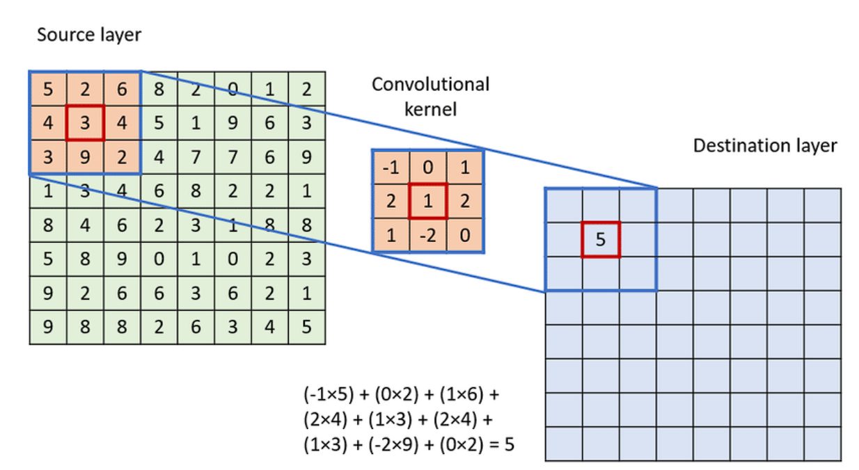
This process has two key properties that make it efficient and powerful:

• Locality: The output at a certain position depends only on a small region of the input (the receptive field).
• Parameter Sharing: The same kernel is used across the entire input, allowing the network to detect the same feature (e.g., an edge, a corner) regardless of where it appears.

For a more detailed breakdown of how convolutions work, including concepts like stride and padding, please review the following slides.

Interestingly, a convolution can be mathematically transformed into a very large, but very sparse, matrix multiplication (this is called im2col). The next video segment builds a beautiful intuition for how convolution is related to matrix multiplication by leveraging the properties of locality and stationarity.

From Abstract Operations to Hardware Kernels

As a systems engineer, it's crucial to understand how these high-level concepts translate to what the machine actually executes. When you write model(input) in PyTorch, the framework doesn't run a slow, Python-based loop for the convolution. Instead, it calls highly optimized, pre-compiled functions from a specialized library.

This is where the term kernel (in the GPU programming sense, not the convolution filter sense) comes in.

So, the performance of your AI workload is ultimately determined by the efficiency of the underlying cuDNN kernels that execute the GEMM and convolution operations on the GPU. Your observability tool will need to monitor the execution of these kernels.

Other Important Operations

While GEMM and convolution are the heavyweights, other operations complete the picture. You'll see these as distinct layers in a model architecture.

• Activation Functions (e.g., ReLU, Sigmoid): Element-wise operations applied after a convolution or linear layer. They are computationally cheap but executed very frequently.
• Pooling Layers (e.g., MaxPooling, AveragePooling): Reduce the spatial dimensions of the data (down-sampling), which helps control the number of parameters.
• Normalization Layers (e.g., BatchNorm): Stabilize training by normalizing the outputs of a previous layer.

The diagram below shows how these different computational blocks (Conv2D, BatchNorm, ReLU, Pooling, Fully Connected) are arranged in a typical Convolutional Neural Network (CNN).

import torch.nn as nn

model = nn.Sequential(
    nn.Conv2d(in_channels=3, out_channels=16, kernel_size=3, stride=1, padding=1),
    nn.ReLU(),
    nn.MaxPool2d(kernel_size=2, stride=2),
    nn.Flatten(),
    nn.Linear(in_features=16*112*112, out_features=10) # Assuming 224x224 input
)

Conclusion

In this lesson, we peeled back another layer of abstraction to identify the core computations that drive deep learning workloads.

Key Takeaways:

• The two most computationally dominant operations in deep learning are Matrix Multiplication (GEMM) and Convolution.
• GEMM is the foundation of fully-connected layers, while Convolution is central to models that process spatial data, like images.
• These high-level operations are implemented as highly optimized, parallel kernels (e.g., from the cuDNN library) that run on the GPU.
• Other operations like activations, pooling, and normalization are also important but typically consume far fewer resources.

You now understand what is being computed during the forward and backward passes. This knowledge is the bedrock for performance analysis. In our next lesson, we will explore the role of batch size, a critical hyperparameter that directly influences the size of the matrices and tensors involved in these operations, and thus has a profound impact on throughput and resource utilization.