Analyzing Loop Time Complexity

The Basic Principle of Loop Analysis

Analyzing a loop's complexity boils down to a simple formula:

Total Time = (Number of Iterations) × (Complexity of Operations Inside the Loop)

For the loops we'll study today, we'll assume the operations inside the loop are "basic"—things like arithmetic, assignments, or simple comparisons. These are constant time, or O(1), operations. Therefore, our main job is to accurately count the number of iterations the loop performs in the worst-case scenario.

To get a formal overview of this process, please take a look at the following reading.

1. Single Loops: Linear Time Complexity — O(n)

The most straightforward case is a single loop that iterates over a collection of size n.

Consider this simple loop written in Rust:

fn print_items(n: i32) {
    for i in 0..n { // This loop runs 'n' times
        // This is an O(1) operation
        println!("Item: {}", i);
    }
}

Here's the analysis:

1. Number of Iterations: The loop runs from 0 up to (but not including) n. This gives us n iterations.
2. Complexity Inside: The println! macro is a single operation. We consider it O(1).
3. Total Time: n iterations × O(1) per iteration = O(n).

This is called linear time complexity. If the input n doubles, the number of operations roughly doubles.

What about loops that look slightly different? For example, a loop that decrements, or one that skips items? The following video provides a concise analysis of these common variations.

The key insight is that whether a loop runs n times, n/2 times, or n/20 times, its growth rate is still directly proportional to n. In Big O notation, they all simplify to O(n).

2. Nested Loops: Quadratic Time Complexity — O(n²)

Things get more interesting when we place loops inside other loops. This is a very common pattern, especially when dealing with 2D structures like grids or when comparing every element in a collection to every other element.

Case 1: Independent Nested Loops

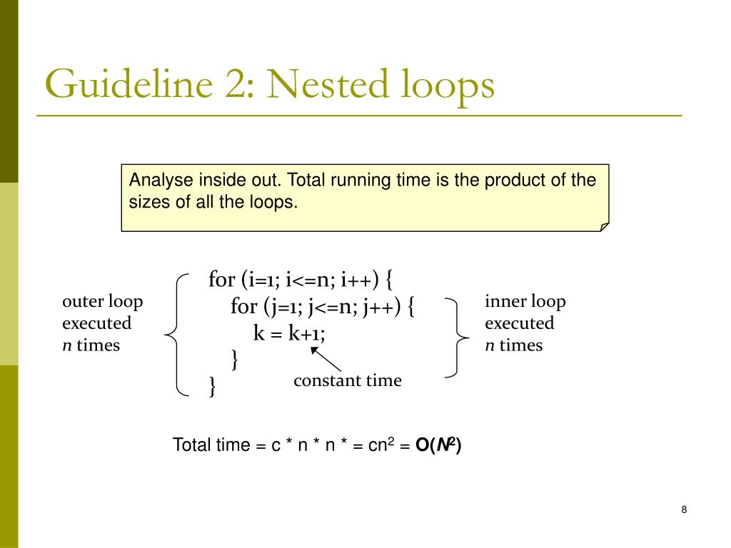
This is the classic O(n²) case where the inner loop's iterations do not depend on the outer loop's variable.

fn print_pairs(n: i32) {
    for i in 0..n { // Outer loop runs 'n' times
        for j in 0..n { // Inner loop runs 'n' times for EACH outer iteration
            // O(1) operation
            println!("Pair: ({}, {})", i, j);
        }
    }
}

Analysis:

1. The outer loop runs n times.
2. For each of those n iterations, the inner loop runs n times.
3. Total Time: n (outer) × n (inner) × O(1) (body) = O(n²).

This is called quadratic time complexity. If n doubles, the runtime quadruples (2²=4). This can become slow very quickly as n grows.

The NeetCode video you saw in the last lesson has an excellent segment explaining this for 2D arrays, which is a perfect real-world example.

Case 2: Dependent Nested Loops

A slightly more complex, but equally common, pattern is when the inner loop's number of iterations depends on the outer loop's current variable.

fn print_lower_triangle(n: i32) {
    for i in 0..n {      // Outer loop runs 'n' times
        for j in 0..i {  // Inner loop's iterations depend on 'i'
            // O(1) operation
            println!("Pair: ({}, {})", i, j);
        }
    }
}

How do we analyze this? We can't simply multiply n * n. Let's trace the number of inner loop iterations for each value of i:

• When i = 0, the inner loop runs 0 times.
• When i = 1, the inner loop runs 1 time (j=0).
• When i = 2, the inner loop runs 2 times (j=0, 1).
• ...
• When i = n-1, the inner loop runs n-1 times.

The total number of operations is the sum of an arithmetic series: 0 + 1 + 2 + ... + (n-1).
This sum has a well-known formula: (n-1) * n / 2.

Expanding this gives (n² - n) / 2 = 0.5n² - 0.5n.

Applying our Big O simplification rules from the last lesson:

1. Drop lower-order terms: O(0.5n² - 0.5n) becomes O(0.5n²).
2. Drop constants: O(0.5n²) becomes O(n²).

Even though it does roughly half the work of the independent nested loop, it has the same quadratic growth rate. Dr. Bari's video provides a fantastic, detailed trace of exactly this scenario.

3. Consecutive Loops: Additive Complexity — O(n + m)

What if loops are not nested, but run one after the other?

fn two_separate_loops(n: i32, m: i32) {
    for i in 0..n {
        // O(1) operation
        println!("First loop: {}", i);
    }

    for j in 0..m {
        // O(1) operation
        println!("Second loop: {}", j);
    }
}

In this case, we simply add the complexities:

• The first loop is O(n).
• The second loop is O(m).
• Total Time: O(n) + O(m) = O(n + m).

If both loops run n times, the complexity is O(n) + O(n) = O(2n), which simplifies to O(n). When complexities are added, the final Big O is determined by the dominant (largest) term. For example, a nested loop followed by a single loop (O(n²) + O(n)) simplifies to O(n²).

Key Takeaways

• Single Loop: A loop that iterates n times has O(n) complexity, assuming its body is O(1).
• Independent Nested Loops: An outer loop running n times and an inner loop running m times results in O(n * m) complexity. If both run n times, it's O(n²).
• Dependent Nested Loops: A common pattern where the inner loop runs i times (where i is the outer loop index) also results in O(n²), due to the sum of an arithmetic series.
• Consecutive Loops: The complexities are added, e.g., O(n) + O(m) = O(n + m). The final Big O is determined by the highest-order term.

Next Steps

You can now look at basic loop structures and determine their time complexity. This is the bedrock of algorithm analysis.

In the next lesson, we will shift our focus from time to memory. You will learn to calculate the space complexity of algorithms, which measures how much auxiliary memory an algorithm uses as its input size grows.