Understanding Big O Notation

What is Big O Notation? The Language of Scalability

At its core, Big O notation is a way to describe how an algorithm's performance changes as the size of its input grows. Think of it as a tool for analyzing an algorithm's scalability at a micro level, much like you would analyze a service's scalability at a macro level.

Instead of measuring performance in seconds or milliseconds, which can vary wildly depending on the hardware, programming language, or current system load, Big O provides a standardized, abstract way to talk about efficiency. It focuses on the growth rate of the work an algorithm does.

To get a quick and clear introduction to this idea, please watch the first part of the following video.

Simplifying the Math

As the video mentioned, a key aspect of Big O analysis is simplification. We are interested in the "big picture" of how an algorithm behaves as the input size, which we'll call n, becomes very large. This means we can ignore parts of our analysis that become insignificant as n grows.

There are two main rules for simplification:

1. Drop Constants: An algorithm that takes 2n steps is in the same complexity class as one that takes n steps. We simplify O(2n) to O(n). The constant factor 2 doesn't change the fundamental linear growth rate.
2. Drop Lower-Order Terms: If an algorithm takes n² + n steps, the n² term will dominate the n term as n gets large. For n = 1,000,000, n² is a trillion, while n is "only" a million. The + n part is negligible in comparison. Therefore, we simplify O(n² + n) to O(n²).

To see this principle illustrated with clear tables and examples, please read the first few sections of the following article.

Why Does Big O Matter for Interviews and Engineering?

Your experience with systems like Redis has already shown you the power of efficient operations. The reason a Redis lookup is so fast is because its underlying data structure (a hash table) provides, on average, O(1) or constant time access. This means the time to find a key is independent of how many keys are in the database.

This is the practical impact of Big O. Understanding it allows you to:

• Compare Solutions: Objectively compare two different algorithms for the same problem and predict which will be more efficient at scale.
• Make Design Decisions: Choose the right data structures and algorithms for a task. Using a list (O(n) search) where a hash set (O(1) average search) is needed can be the difference between a snappy feature and a slow, unusable one.
• Communicate with Engineers: Use a shared, precise language to discuss code performance.
• Demonstrate Seniority in Interviews: Interviewers use Big O questions to see if you think about the long-term consequences and scalability of your code, a key differentiator for senior roles.

The article you just looked at has a section that speaks directly to your goal of interview preparation.

A Tour of Common Big O Complexities

Algorithms are categorized into different "complexity classes." Seeing how they compare visually is powerful. As input size n grows, the difference between an efficient and an inefficient algorithm becomes dramatic.

Let's explore the most common classes you'll encounter, from best to worst. The NeetCode video you started earlier gives excellent, code-centric examples for each one.

Building Intuition: The Bookshelf Metaphor

Analogies can help solidify these abstract concepts. The following resource provides an excellent, intuitive metaphor for each complexity class using the simple task of organizing a bookshelf.

One last point: Big O notation technically describes the worst-case scenario. While there are other notations for best-case (Big Omega, Ω) and average-case (Big Theta, Θ), the industry and interviews overwhelmingly focus on the worst-case Big O. It provides a guarantee: your algorithm will perform at least this well, and no worse.

Here is a useful cheat sheet that summarizes the main complexity classes with examples.

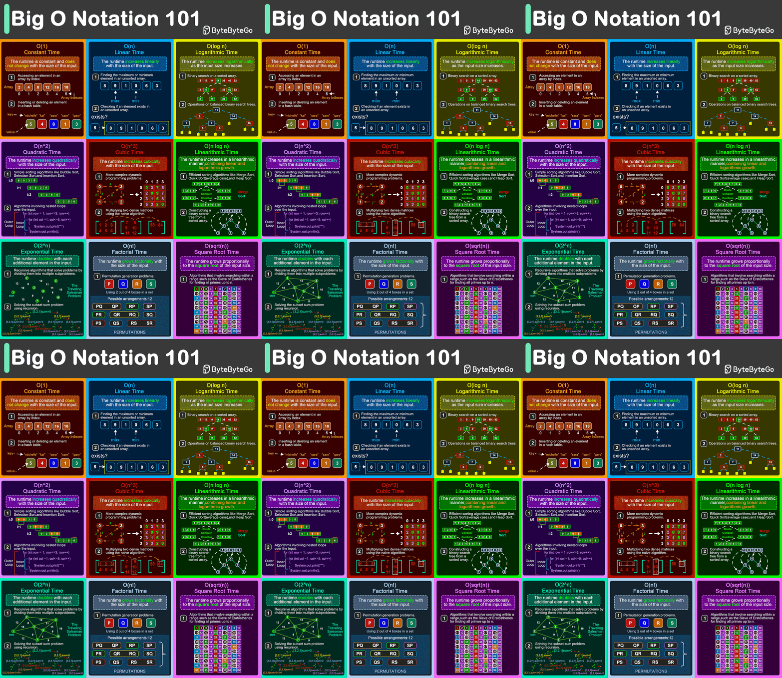
Key Takeaways

• Big O describes scalability: It measures how an algorithm's runtime or space requirements grow as the input size (n) increases.
• It's an abstraction: It ignores hardware specifics, clock time, constants, and lower-order terms to focus on the fundamental growth rate.
• It's essential for comparison: Big O provides a standard way to analyze and compare the efficiency of algorithms, which is critical for making informed engineering decisions and for technical interviews.
• Common classes range from great to terrible: You'll most often encounter O(1), O(log n), O(n), O(n log n), and O(n²). Exponential O(2ⁿ) and factorial O(n!) complexities are generally too slow for large inputs.

On to the Next Step

In this lesson, we've defined what Big O is and why it matters. You now have the conceptual framework.

In the next lesson, we will start applying this knowledge directly to code. You will learn to calculate the time complexity of simple loops and nested loops, our first practical step in analyzing algorithms. This will be the foundation for evaluating every piece of code we write in this course.