Auxiliary Space Complexity

1. What is Space Complexity? The Key Distinction

Just as time complexity describes how runtime grows with input size, space complexity describes how memory usage grows. However, there's a crucial distinction you need to make, especially for interviews.

An algorithm's total memory footprint consists of two parts:

1. Input Space: The memory used to store the input data itself. For example, if your function receives an array of n integers, the input space is O(n).
2. Auxiliary Space: The extra or temporary memory that the algorithm uses during its execution. This includes variables, data structures created inside the function, and the space taken by the function call stack.

In algorithm analysis and coding interviews, when we talk about "space complexity," we are almost always referring to the auxiliary space. Why? Because we want to measure the memory cost of the algorithm itself, not the memory required to simply hold the data it's processing.

To solidify this distinction, please read the following short article. It provides a direct and clear comparison.

2. Calculating Auxiliary Space Complexity

Now, let's practice calculating this auxiliary space for different scenarios.

Constant Space Complexity: O(1)

An algorithm has O(1) auxiliary space complexity if the amount of extra memory it needs does not change with the input size. This is typical for algorithms that only use a few simple variables to do their work.

Consider the array-summing example from the article you just read, here written in Rust:

fn sum_array(arr: &[i32]) -> i32 {
    let mut sum = 0; // One integer variable: O(1)
    // The loop counter 'i' is created internally by the iterator.
    // It's also O(1) space.
    for &item in arr {
        sum += item;
    }
    sum
}

• Input Space: The input arr takes O(n) space, where n is the number of elements.
• Auxiliary Space: The algorithm only creates one extra variable, sum, to hold the result. The memory for this variable is fixed, regardless of whether the array has 10 elements or 10 million. Therefore, the auxiliary space complexity is O(1).

Let's watch a short video that analyzes a similar algorithm, linear search, which also has O(1) auxiliary space despite its O(n) time complexity.

Linear Space Complexity: O(n)

An algorithm has O(n) auxiliary space complexity if the extra memory it uses grows linearly with the input size n. This typically happens when you create a new data structure that is a copy of the input or has a size proportional to it.

Here’s a Rust function that creates a new vector containing the doubled values of an input slice:

fn double_elements(arr: &[i32]) -> Vec<i32> {
    // We allocate a new vector with the same capacity as the input array.
    // This is O(n) auxiliary space.
    let mut new_arr = Vec::with_capacity(arr.len());

    for &item in arr {
        new_arr.push(item * 2);
    }
    new_arr // The returned vector's memory was allocated by the algorithm.
}

In this case, the new_arr vector is the auxiliary space. Since its size is directly proportional to the size of the input arr, the auxiliary space complexity is O(n).

Space Complexity of Recursion: The Call Stack

Recursion presents a less obvious source of space complexity: the function call stack. Each time a function calls itself, a new stack frame is created in memory to store its local variables, arguments, and the return address. The maximum depth of the call stack during the execution determines the space complexity of the recursion.

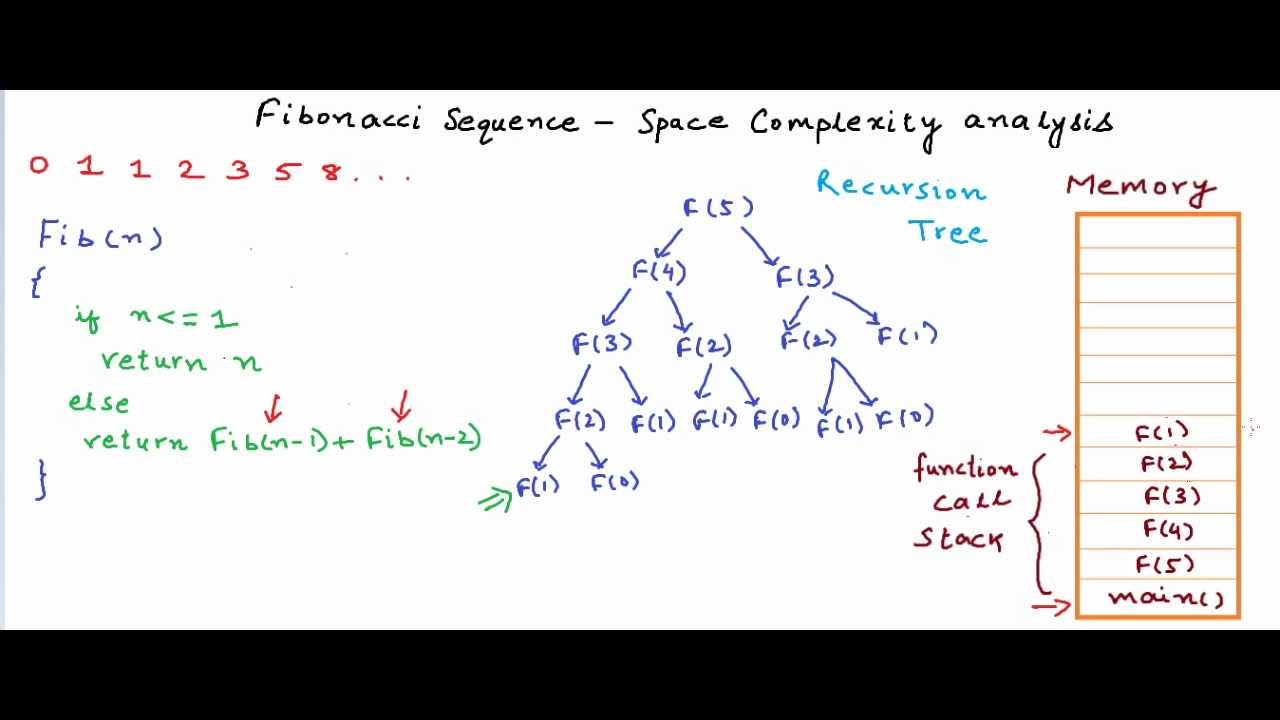
The following video provides an excellent, detailed walkthrough of how the call stack grows when executing a recursive factorial function, leading to O(n) space complexity.

This is a critical concept. While an iterative factorial solution would have O(1) auxiliary space, the naive recursive version has O(n) auxiliary space due to the stack depth.

Not all recursion is O(n). For example, a recursive binary search algorithm would have O(log n) space complexity because it halves the input at each step, so the stack depth grows logarithmically. We'll explore this further in the sorting and searching module.

3. The Time-Space Trade-off

As an experienced engineer, you intuitively know that there are no free lunches. Often, you can make an algorithm faster by using more memory, or reduce its memory footprint at the cost of more computation time. This is the classic time-space trade-off. Understanding this trade-off is key to making informed architectural decisions.

The following resource discusses this concept with clear examples.

This trade-off is a recurring theme in algorithm design. Using a hash map to cache results or count frequencies is a perfect example: you accept O(n) space to achieve O(1) lookups, a trade you'll make frequently in solving LeetCode problems.

Conclusion

You've now added another critical dimension to your analysis toolkit. Understanding how to evaluate memory usage is just as important as analyzing runtime.

Key Takeaways:

• Space Complexity measures how an algorithm's memory usage scales with input size.
• We primarily focus on Auxiliary Space: the extra memory an algorithm uses, excluding the input itself.
• O(1) space is constant extra space, typical for algorithms using only primitive variables.
• O(n) space is linear extra space, often from creating a new data structure whose size depends on the input.
• Recursion consumes space on the call stack. The space complexity is determined by the maximum depth of recursion, which can be O(n) (like factorial) or O(log n) (like binary search).
• Algorithm design often involves a time-space trade-off, where you can sacrifice memory for speed or vice-versa.

Next Steps

In this and the previous lessons, you've learned to calculate complexity for both time (O(1), O(n), O(n²)) and space (O(1), O(log n), O(n)). In our next lesson, we will formalize the comparison of these common complexity classes. You'll learn to rank them, understand their growth rates more deeply, and be able to quickly judge the theoretical efficiency of an algorithm.