Rolling Window Statistics for Time-Series Data

1. The Concept of a Rolling Window

Before diving into the code, let's establish the intuition. A "rolling" or "moving" calculation applies an operation to a sliding window of data. Imagine you have a time series of daily prices. A 10-day rolling calculation would first look at days 1-10 and compute a value (e.g., the average). Then, the window "rolls" forward one step: it looks at days 2-11 and computes the average. This process continues until the end of the series, creating a new time series of the calculated statistic.

This technique is powerful because it allows us to see how a metric evolves over time, rather than just calculating a single value for the entire dataset. In Pandas, the .rolling() method is our primary tool for this.

2. Smoothing the Trend: Moving Averages

A Simple Moving Average (SMA) is the most common rolling statistic. It calculates the average price over a specific number of preceding periods, serving to smooth out price data and make it easier to identify the underlying trend.

To understand how this is implemented and why it's useful, let's watch a short video that explains the rolling method in Pandas to calculate an SMA.

As the video demonstrated, calculating an SMA in Pandas is elegantly simple. If you have a DataFrame df with a Close column, a 50-day SMA is just one line:

df['SMA50'] = df['Close'].rolling(window=50).mean()

The .rolling(window=50) part creates the sliding window object, and .mean() is the aggregation function applied to each window. The result is a new Series containing the 50-day SMA, which we can assign to a new column.

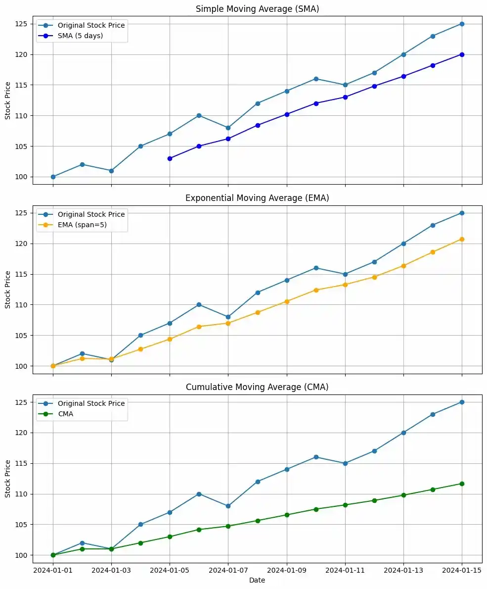
The smoothing effect of different types of moving averages is clearly visible when plotted against the original price series.

3. Quantifying Risk: Historical Volatility

While moving averages help with trend, historical volatility (HV) helps us understand risk. It measures the dispersion of returns for a given security over a specific period. Formally, it is the standard deviation of returns.

Calculating rolling historical volatility follows a three-step process:

1. Calculate Returns: First, we need a time series of asset returns. As we learned previously, daily log returns or simple percentage returns are standard. df['Close'].pct_change() is perfect for this.
2. Calculate Rolling Standard Deviation: We then apply the .rolling() method to the returns series, this time using .std() as our aggregation function to get the rolling standard deviation.
3. Annualize the Volatility: The result from step 2 is a standard deviation of daily returns. To make it comparable across different timeframes, we annualize it. Assuming there are 252 trading days in a year, we do this by multiplying the daily volatility by the square root of 252.

The formula for annualized rolling historical volatility is:

Let's look at a concise article that puts this into code.

The code from the article cleanly implements our three-step process:

# The window is set to 21, representing approximately one month of trading days
window_size = 21




# 1. pct_change() calculates returns
# 2. .rolling().std() calculates rolling standard deviation
# 3. * math.sqrt(252) annualizes it
data['vol'] = data['Close'].pct_change().rolling(window=window_size).std() * math.sqrt(252)

This is the standard approach you will use to measure historical volatility for your trading models.

Now, let's see a video that visualizes this process.

4. Putting It All Together: A Practical Example

Let's combine these concepts into a single script. We will fetch data for the Nifty 50 index, calculate its 50-day SMA and its 21-day rolling historical volatility, and then plot the results.

import yfinance as yf
import pandas as pd
import numpy as np
import matplotlib.pyplot as plt




# Fetch NIFTY 50 data
nifty = yf.download('^NSEI', start='2020-01-01', end='2023-12-31')




# --- Calculate Rolling Statistics ---




# 1. Simple Moving Average (50-day)
nifty['SMA50'] = nifty['Close'].rolling(window=50).mean()




# 2. Historical Volatility (21-day, annualized)
nifty['Log_Return'] = np.log(nifty['Close'] / nifty['Close'].shift(1))
nifty['Volatility'] = nifty['Log_Return'].rolling(window=21).std() * np.sqrt(252)





# --- Visualization ---




# Set up the plot
fig, ax1 = plt.subplots(figsize=(14, 7))




# Plot Close Price and SMA50 on the primary y-axis (ax1)
ax1.set_xlabel('Date')
ax1.set_ylabel('Price (INR)', color='tab:blue')
ax1.plot(nifty.index, nifty['Close'], color='tab:blue', label='NIFTY 50 Close')
ax1.plot(nifty.index, nifty['SMA50'], color='orange', linestyle='--', label='50-Day SMA')
ax1.tick_params(axis='y', labelcolor='tab:blue')
ax1.legend(loc='upper left')
ax1.grid(True)




# Create a secondary y-axis for Volatility
ax2 = ax1.twinx()
ax2.set_ylabel('Annualized Volatility', color='tab:red')
ax2.plot(nifty.index, nifty['Volatility'], color='tab:red', label='21-Day HV')
ax2.tick_params(axis='y', labelcolor='tab:red')
ax2.legend(loc='upper right')




# Show the plot
fig.tight_layout()
plt.title('NIFTY 50 Price and Rolling Volatility')
plt.show()




# Display the last few rows of the DataFrame
print(nifty.tail())

Interpreting the Output:
When you run this code, you will see a plot showing the NIFTY 50's price alongside its moving average, with the historical volatility plotted below it on a separate scale. Notice how the volatility (red line) spikes during periods of large price swings (like the COVID-19 crash in early 2020) and subsides during calmer market periods.

You'll also notice NaN (Not a Number) values at the beginning of the SMA50 and Volatility columns. This is expected. The first valid 50-day SMA can only be calculated on the 50th day, as it needs 50 data points. Similarly, the first volatility value requires 21 days of returns.

Conclusion

In this lesson, you have translated core financial concepts into practical, vectorized Python code. You are now equipped to quantify two of the most important market dynamics: trend and volatility.

Key Takeaways:

• The .rolling() method in Pandas is the key to calculating moving statistics on time-series data.
• A Simple Moving Average (SMA) is calculated with .rolling(window=...).mean() and is used to smooth price data to identify trends.
• Annualized Historical Volatility is calculated by taking the rolling standard deviation of returns (.rolling(window=...).std()) and scaling it by the square root of 252.
• These rolling metrics are dynamic—they evolve with the market, providing a timely view of trend and risk, which is crucial for algorithmic trading.

Preview of the Next Lesson:
We've had a taste of fetching data with yfinance. In the next lesson, we will formalize this process. We'll explore how to reliably fetch historical market data using APIs and prepare it for analysis, ensuring you have a robust data pipeline, which is the true starting point for any quantitative research project.