Vectorized Financial Data Analysis with NumPy and Pandas

1. The Need for Speed: From Loops to Vectorization

In quantitative finance, we often deal with millions of data points, whether they are historical prices, tick data, or simulation outputs. Processing this data efficiently is not just a convenience; it's a necessity. A standard Python for loop, which processes data element-by-element, is often too slow for these tasks.

The solution is vectorization: performing operations on entire arrays (or "vectors") of data at once, rather than iterating through individual elements. This approach delegates the looping to highly optimized, pre-compiled C code that underpins libraries like NumPy and Pandas, leading to dramatic performance gains.

To see a practical demonstration of this, let's watch a video that compares three methods for solving a simple problem in Pandas: a for loop, the .apply() method, and a fully vectorized approach.

As the video clearly shows, vectorization isn't just a minor optimization—it can be thousands of times faster. For a quant trader, this is the difference between a backtest that runs in seconds versus one that runs for hours. This principle will be the bedrock of all the Python code we write in this course.

2. NumPy: The Engine of Numerical Computing

NumPy (Numerical Python) is the foundational library for numerical operations in Python. It introduces the ndarray (n-dimensional array), a powerful data structure for efficient vectorized computations. Pandas DataFrames, which we will cover next, are built directly on top of NumPy arrays.

Let's explore how NumPy's vectorized nature is applied to common financial calculations. We'll draw upon a comprehensive guide that showcases these capabilities.

2.1. Vectorized Return Calculations

As you saw in the reading, calculating returns across a whole time series of prices is a perfect example of vectorization. Instead of looping, we use array slicing and element-wise operations.

Let's say we have an array of prices p:
p = [100, 102, 99, 101]

To calculate simple returns $\frac{P_t}{P_{t-1}}-1$, we can do this in one line with NumPy:

import numpy as np

prices = np.array([100, 102, 99, 101])




# prices[1:] gives [102, 99, 101] (the 'final values')
# prices[:-1] gives [100, 102, 99] (the 'initial values')
simple_returns = prices[1:] / prices[:-1] - 1

print(simple_returns)



# Output: [ 0.02      -0.02941176  0.02020202]

Similarly, log returns $\ln (\frac{P_t}{P_{t-1}})$ are just as simple:

log_returns = np.log(prices[1:] / prices[:-1])

print(log_returns)



# Output: [ 0.01980263 -0.02985333  0.02      ]

This is significantly more efficient and readable than writing a loop.

2.2. Universal Functions and Descriptive Statistics

NumPy provides a rich set of "ufuncs" (universal functions) that operate element-wise on arrays. This includes mathematical functions like np.log(), np.exp(), and np.sqrt(), as well as aggregation functions like np.mean(), np.sum(), and np.std().

When working with multi-dimensional arrays (like a matrix of returns for several stocks), you can specify the axis argument to perform aggregations along rows or columns.

• axis=0 computes the statistic down the columns.
• axis=1 computes the statistic across the rows.

For a typical financial data matrix where rows are stocks and columns are time periods, axis=1 is used to get per-stock statistics over time.

A Critical Note on Standard Deviation:

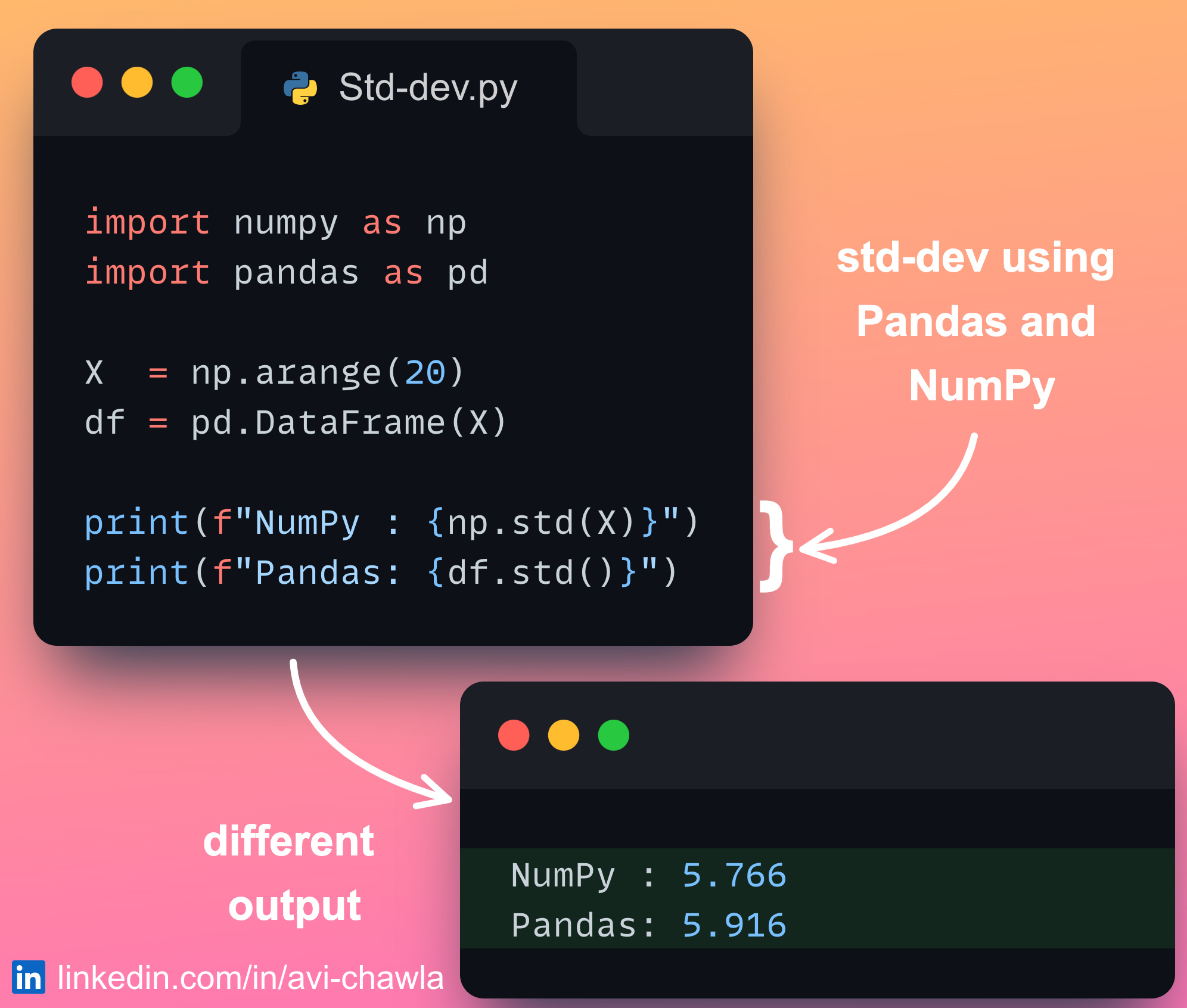
A common pitfall is the difference in default behavior between NumPy's and Pandas' standard deviation calculation. By default, NumPy calculates the population standard deviation, while Pandas calculates the sample standard deviation. In finance, we almost always work with a sample of data, so we need the latter.

To make NumPy compute the sample standard deviation, you must specify ddof=1 (delta degrees of freedom).

3. Pandas: Your Primary Tool for Financial Data

While NumPy is the engine, Pandas is the vehicle. It provides two primary data structures that are indispensable for a quant: the Series (a single column) and the DataFrame (a table). Think of a DataFrame as an Excel spreadsheet on steroids, with powerful indexing, time-series functionality, and data alignment capabilities.

The typical workflow in quantitative finance using Pandas is nicely summarized in this diagram.

Let's focus on the core manipulations you'll perform daily.

3.1. Selecting and Filtering Data

One of Pandas' greatest strengths is its rich API for selecting subsets of data. You'll use this constantly to filter for specific assets, dates, or conditions.

To summarize the key methods:

• .iloc[]: Selects data by integer position (e.g., df.iloc[0, 5] for the first row, sixth column).
• .loc[]: Selects data by label (e.g., df.loc['2023-10-25', 'AAPL'] for a specific date and stock).
• Boolean Indexing: The most powerful method. You provide a Series of True/False values to filter rows. For example, to find all days where NIFTY closed up more than 1%: df.loc[df['Close'] > df['Close'].shift(1) * 1.01].

3.2. Essential Time-Series Manipulations

For trading strategy development, you almost always need to compare values at different points in time. Pandas makes this trivial with its time-series manipulation methods.

Shifting Data (.shift()):
The .shift() method is fundamental. It shifts the data in a Series or DataFrame forward or backward by a specified number of periods. This is how you access lagged values to calculate returns, momentum, and other time-series indicators without loops.

For example, df['Close'].shift(1) creates a new series where each element is the closing price from the previous day. This is the key building block for vectorized return calculations in Pandas:

# Assume 'df' is a DataFrame with a 'Close' column indexed by date
df['Yesterday_Close'] = df['Close'].shift(1)
df['Simple_Return'] = (df['Close'] / df['Yesterday_Close']) - 1

Pandas provides a shortcut for this specific operation: .pct_change().

df['Simple_Return'] = df['Close'].pct_change()

This single line does the same work as the manual shift and division, handling the NaN value for the first row automatically.

A Look-Ahead Example:
The following video demonstrates a more advanced use of .shift() to create multiple look-ahead columns for a vectorized backtest. We won't build the full backtester now, but seeing the technique is highly instructive.

This technique of shifting data to align past or future values with the current time step is a cornerstone of vectorized strategy implementation.

4. A Practical Walkthrough

Let's tie this together with a quick, practical example using yfinance to grab data and Pandas/NumPy to manipulate it.

import yfinance as yf
import pandas as pd
import numpy as np




# 1. Fetch historical data for the NIFTY 50 index
data = yf.download('^NSEI', start='2022-01-01', end='2023-12-31')




# 2. Calculate simple returns using the vectorized pct_change() method
data['simple_return'] = data['Adj Close'].pct_change()




# 3. Calculate log returns using NumPy's log function on the simple returns
# We add 1 to the simple return before taking the log
data['log_return'] = np.log(1 + data['simple_return'])




# 4. Use boolean indexing to filter for days with a large move (> 2%)
large_moves = data[data['simple_return'].abs() > 0.02]




# 5. Display the first few rows of the original dataframe with new columns
print("Data with returns:")
print(data.head())




# 6. Display the filtered dataframe of large moves
print("\nDays with large moves (> 2%):")
print(large_moves)

In this short script, you can see how we fluidly combine Pandas for data handling (creating columns, indexing) and NumPy for a mathematical operation (np.log). This interplay is typical in quantitative analysis.

Conclusion

This lesson moved us from the "what" of financial models to the "how" of their implementation. Mastering vectorized computation with NumPy and Pandas is a non-negotiable skill for any aspiring quant.

Key Takeaways:

• Vectorization is King: Always prefer vectorized operations on whole arrays/columns over row-by-row loops for performance.
• NumPy is the Foundation: It provides the core ndarray object and fast mathematical functions for numerical heavy lifting.
• Pandas is the Workbench: Its DataFrame is the primary tool for handling and manipulating labeled, time-indexed financial data.
• Core Skills: You are now equipped to select, filter, and perform time-series manipulations like calculating returns and shifting data—the essential building blocks for strategy development.

Preview of the Next Lesson:
We will immediately build on today's skills. The next lesson focuses on calculating rolling window statistics, such as moving averages and historical volatility. You will learn to use methods like .rolling() to compute these key indicators in a vectorized way, which are fundamental inputs for many trading strategies.