Hubbard Model: Hopping and Interaction

From Concepts to Operators

In the previous lesson, we saw how $t$ and $U$ arise as matrix elements of the full electronic Hamiltonian when expressed in a localized Wannier basis. Now, we'll write the simplified model Hamiltonian that retains only these dominant terms. To do this, we use the fermionic creation ($c_{i\sigma }^{†}$) and annihilation ($c_{i\sigma }$) operators, which create or destroy an electron with spin $\sigma$ at a specific lattice site $i$.

The excellent introductory notes by Richard Scalettar provide a very clear and self-contained description of how these operators are used to construct the Hubbard Hamiltonian.

Deconstructing the Hubbard Hamiltonian

As you saw in the reading, the Hubbard Hamiltonian consists of two parts, corresponding to the two competing physical processes we've discussed. Let's write it down and examine each term in detail.

The full Hubbard Hamiltonian is:

1. The Kinetic Term: Hopping

The first part of the Hamiltonian is the kinetic energy term, which you'll recognize from our study of the tight-binding model:

Let's break this down:

• $c_{j\sigma }$: This operator annihilates an electron with spin $\sigma$ at site $j$.
• $c_{i\sigma }^{†}$: This operator creates an electron with the same spin $\sigma$ at site $i$.
• $c_{i\sigma }^{†}{c}_{j\sigma }$: The combined operation describes the "hopping" or "tunneling" of an electron from site $j$ to site $i$.
• ${\sum }_{⟨i,j⟩}$: This sum is restricted to nearest-neighbor pairs of sites. This is a standard and often excellent approximation, as the overlap of atomic wavefunctions (which determines the hopping probability) decays exponentially with distance.
• $-t$: The parameter $t$, called the hopping integral or hopping parameter, sets the energy scale for this kinetic process. A positive $t$ means that the system's energy is lowered when electrons are delocalized and can move freely between sites. The negative sign ensures this energy lowering. The term $c_{j\sigma }^{†}{c}_{i\sigma }$ is the Hermitian conjugate, ensuring the Hamiltonian is a Hermitian operator as required.

This term promotes metallic behavior. It favors wavefunctions where electrons are spread across the entire lattice, minimizing their kinetic energy.

2. The Interaction Term: On-Site Repulsion

The second part of the Hamiltonian is the new ingredient that takes us beyond the simple tight-binding model:

Here's the breakdown:

• ${\hat{n}}_{i\sigma }=c_{i\sigma }^{†}{c}_{i\sigma }$: This is the number operator. It gives 1 if a state has an electron with spin $\sigma$ at site $i$, and 0 otherwise.
• ${\hat{n}}_{i\uparrow }{\hat{n}}_{i\downarrow }$: This product of number operators acts as a "double-occupancy detector". It yields 1 only if site $i$ is occupied by both a spin-up electron and a spin-down electron. If the site is empty, or singly occupied, the product is 0.
• $U$: The parameter $U$ is the on-site Coulomb repulsion. It sets the energy cost for putting two electrons on the same site. For $U>0$, this term penalizes double occupancy.

This term promotes insulating behavior. To minimize this energy, electrons will tend to avoid each other by occupying different sites, leading to localization. The derivation in the TCM Group notes, which you saw in the previous lesson, formally justifies this term as the dominant part of the full Coulomb interaction in a localized basis. The final result is concisely stated just before Equation (2.12).

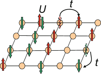
The Competition Visualized

The entire physics of the Hubbard model emerges from the battle between these two terms. The parameter $t$ encourages electrons to delocalize to lower their kinetic energy, while the parameter $U$ forces them to localize to avoid a large potential energy penalty. The ratio $U/t$ becomes the crucial dimensionless parameter that dictates the behavior of the system.

The image below provides a perfect visual summary of these two competing processes on a lattice.

Finally, it's worth noting that the Hamiltonian is often written with a third term, the chemical potential:

The chemical potential $\mu$ acts as a control knob for the total number of electrons (the filling) in the system, which is essential when working in the grand canonical ensemble. For now, we will mostly work with a fixed number of electrons, so you can consider $\mu$ to be set implicitly.

Conclusion

In this lesson, we have translated the physical concepts of hopping and on-site repulsion into a precise, second-quantized Hamiltonian. This equation, despite its simple appearance, holds a universe of complex many-body phenomena.

Key Takeaways:

• The Hubbard Hamiltonian is composed of a kinetic term and a potential energy term: $\hat{H}={\hat{H}}_t+{\hat{H}}_U$.
• The hopping term, scaled by $t$, describes the delocalization of electrons between nearest-neighbor sites and favors metallic behavior. It is mathematically identical to the tight-binding Hamiltonian.
• The interaction term, scaled by $U$, adds an energy penalty for doubly occupying a single lattice site and favors insulating behavior. It is expressed as $U{\sum }_i{\hat{n}}_{i\uparrow }{\hat{n}}_{i\downarrow }$.
• The fundamental physics of the model is governed by the competition between these two terms, encapsulated in the ratio $U/t$.

Now that we have the model's equation and understand its parameters, we can start exploring its behavior. In the next lesson, we will investigate the key physical regimes of the Hubbard model by considering the limits of weak coupling ($U\ll t$) and strong coupling ($U\gg t$), particularly at the important case of half-filling.