Array Manipulation: Indexing, Slicing, and Reshaping

Indexing: Accessing Single Elements

Just like with Python lists, you can access individual elements of a NumPy array using their index. The key difference and improvement comes when working with multi-dimensional arrays.

• 1D Arrays: Works exactly like a Python list. arr[i] gets the element at index i. Remember that indexing starts at 0.
• 2D Arrays (Matrices): You can use a single set of square brackets with a comma to specify the row and column: arr[row, col]. This is cleaner and more efficient than the nested bracket syntax used for lists (my_list[row][col]).

Let's watch a short video that demonstrates this clearly.

Here's a code example to summarize:

import numpy as np

# A 2D array (3 rows, 4 columns)
a = np.array([[1, 2, 3, 4],
              [5, 6, 7, 8],
              [9, 10, 11, 12]])

# Access the element in the 2nd row (index 1) and 3rd column (index 2)
element = a[1, 2]
print(f"Element at [1, 2] is: {element}") # Output: 7

# Negative indexing: access the last element in the first row
last_element_first_row = a[0, -1]
print(f"Element at [0, -1] is: {last_element_first_row}") # Output: 4

# You can also modify elements using indexing
a[0, 0] = 99
print("\nArray after modification:")
print(a)

Slicing: Selecting Subsets of Arrays

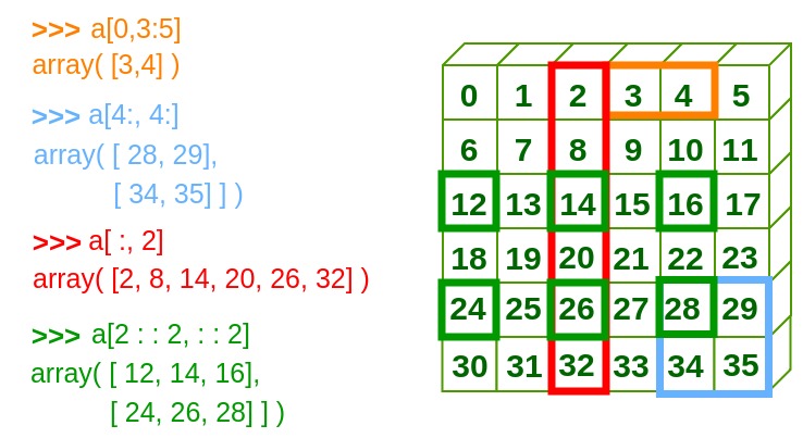
Slicing lets you select entire sections of an array. The syntax is start:stop:step, which should be familiar from Python lists. Where NumPy shines is applying this across multiple dimensions.

The general syntax for a 2D array is arr[row_slice, column_slice]. A single colon : is used to select all elements along that axis.

• a[1, :] or a[1]: Selects the entire second row (index 1).
• a[:, 2]: Selects the entire third column (index 2).
• a[0:2, 1:3]: Selects a sub-array from the first two rows (0 and 1) and the middle two columns (1 and 2).

This image provides a great visual guide to slicing operations.

An Important Distinction: Views vs. Copies

This is a critical concept. When you slice a Python list, you get a new list—a copy of the original data. In NumPy, slicing creates a view of the original array. A view is not a new array; it's a window into the original array's data.

Why does this matter?

1. Performance: Creating views is much faster and more memory-efficient than copying data, especially for large arrays.
2. Side Effects: If you modify a view, you are also modifying the original array. This is a powerful feature but can cause unexpected bugs if you're not aware of it.

If you explicitly need a copy, you must use the .copy() method: new_array = old_array[0:2, :].copy().

a = np.array([[1, 2, 3, 4],
              [5, 6, 7, 8],
              [9, 10, 11, 12]])

Advanced Indexing

Beyond simple slicing, NumPy offers more powerful ways to select data.

1. Boolean Indexing (Masking)

You can use an array of boolean values to select elements. The boolean array (or "mask") must have the same shape as the array you are indexing. This is incredibly useful for filtering data based on conditions.

data = np.array([[10, 25],
                 [30, 15],
                 [40, 5]])

# Create a boolean mask for values greater than 20
mask = data > 20
print("Boolean Mask:\n", mask)
# [[False  True]
#  [ True False]
#  [ True False]]

# Use the mask to select only the elements that are True
print("\nElements greater than 20:\n", data[mask]) # Output: [25 30 40]

2. Integer Array Indexing ("Fancy" Indexing)

You can also use lists or NumPy arrays of integers to select specific elements in a non-contiguous way.

arr = np.array([10, 20, 30, 40, 50, 60])

# Select elements at indices 0, 2, and 5
print(arr[[0, 2, 5]]) # Output: [10 30 60]

# For a 2D array, you can select specific rows
matrix = np.array([[1, 2, 3],
                   [4, 5, 6],
                   [7, 8, 9]])
print("\nSelecting rows 0 and 2:\n", matrix[[0, 2], :])

Unlike slicing, advanced indexing always returns a copy of the data, not a view.

Let's see these advanced techniques in action.

Reshaping Arrays

Often, you'll need to change the dimensions of your array. For example, you might have a long 1D array of pixel values that you need to convert into a 2D array representing an image. This is done with the reshape() method.

The fundamental rule of reshaping is: The size of the new array must be identical to the size of the original array. For instance, you can reshape an array of size 12 into (3, 4), (4, 3), (2, 6), (6, 2), or (12, 1), but not (3, 5).

Here is a code example:

# Create a 1D array of 12 elements
a = np.arange(12)
print("Original array:\n", a)
print("Original shape:", a.shape)

# Reshape it into a 3x4 matrix
b = a.reshape(3, 4)
print("\nReshaped array (3x4):\n", b)
print("New shape:", b.shape)

# Flatten a multi-dimensional array back into 1D
# The -1 is a useful trick that tells NumPy to automatically infer the correct dimension.
c = b.reshape(-1)
print("\nFlattened array:\n", c)
print("Flattened shape:", c.shape)

Adding New Dimensions

A common task, especially when preparing data for machine learning models, is to add a new dimension. For instance, you might convert a 1D vector of shape (n,) into a 2D column vector (n, 1) or row vector (1, n). This is essential for linear algebra operations you'll perform later.

You can do this using reshape, but a more convenient syntax is np.newaxis.

# A 1D array
vec = np.array([1, 2, 3])
print(f"Original shape: {vec.shape}")

# Convert to a row vector
row_vec = vec[np.newaxis, :]
print(f"Row vector shape: {row_vec.shape}") # (1, 3)
print(row_vec)

# Convert to a column vector
col_vec = vec[:, np.newaxis]
print(f"Column vector shape: {col_vec.shape}") # (3, 1)
print(col_vec)

Conclusion

Fantastic work today. You've now acquired a powerful toolkit for manipulating NumPy arrays. These skills—indexing to access data, slicing to create views, advanced indexing for filtering, and reshaping to alter structure—form the backbone of almost all data preparation tasks in machine learning.

Key Takeaways:

• Indexing: Use arr[row, col] for precise element access in 2D arrays.
• Slicing: Use start:stop:step notation to select sections of an array. Slicing creates a view, meaning modifications affect the original array. Use .copy() to create an independent copy.
• Advanced Indexing:
  • Boolean masking (arr[arr > 5]) is a powerful way to filter data based on conditions.
  • Integer array indexing (arr[[1, 5, 7]]) selects specific, non-contiguous elements.
• Reshaping: Use arr.reshape(new_shape) to change an array's dimensions. The total number of elements (size) must remain the same. Use np.newaxis to easily add a dimension.

In our next lesson, we will put these skills to use by learning how to apply fast, vectorized mathematical and statistical operations across entire arrays.