NumPy Array Operations

Why NumPy is Fast: Vectorization

Before we dive into the operations themselves, it's important to understand why NumPy is the tool of choice. Your computer science background gives you a unique advantage in appreciating the underlying mechanics.

At its core, NumPy's speed comes from vectorization. Instead of iterating through array elements one by one in Python (which is slow), NumPy passes the entire array to highly optimized, pre-compiled C code. This code can then perform the operation on the entire block of data at once, often leveraging modern CPU features like SIMD (Single Instruction, Multiple Data) that can perform the same operation on multiple data points simultaneously.

This concept of applying an operation to a whole array at once, rather than in a loop, is the essence of writing efficient, "NumPy-onic" code.

Element-wise Arithmetic Operations

The most common operations you'll perform are basic arithmetic. With NumPy, standard operators like +, -, *, /, and ** (for exponentiation) are not applied to the array object itself, but are applied element-wise to the data within it.

This means you can perform an operation on every single element of an array with a simple, readable syntax.

import numpy as np

a = np.arange(1, 6) # Creates an array [1, 2, 3, 4, 5]
print(f"Original array 'a': {a}")

# Array-scalar operations
print(f"a + 2:  {a + 2}")    # Adds 2 to each element
print(f"a * 3:  {a * 3}")    # Multiplies each element by 3
print(f"a ** 2: {a ** 2}")   # Squares each element

# Array-array operations (must have compatible shapes)
b = np.array([10, 20, 30, 40, 50])
print(f"\nOriginal array 'b': {b}")
print(f"a + b: {a + b}")

This element-wise behavior is a direct parallel to vector and matrix operations in linear algebra. Adding a scalar to a vector or adding two vectors of the same dimension follows the exact same component-wise logic.

Broadcasting: Operations on Mismatched Shapes

A natural question arises: what happens if you try to perform an operation between arrays of different shapes, like a 3x3 matrix and a 1x3 vector? This is where NumPy's powerful broadcasting feature comes in.

Broadcasting describes a set of rules by which NumPy handles operations on arrays of different sizes. The smaller array is "broadcast" across the larger array so that they have compatible shapes.

The core rule is that when operating on two arrays, NumPy compares their shapes element-wise, starting from the trailing (rightmost) dimensions. The dimensions are compatible if:

1. They are equal, or
2. One of them is 1.

If these conditions are met, the array with the dimension of size 1 is "stretched" to match the other array's size in that dimension.

Visualizing this helps.

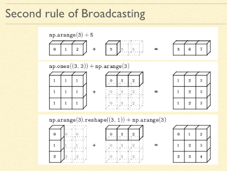
Let's see this in code:

matrix = np.ones((3, 3)) # A 3x3 matrix of all ones
row_vector = np.array([0, 1, 2])

print("Matrix (3x3):\n", matrix)
print("\nRow Vector (1x3):\n", row_vector)

# Broadcasting the row_vector to each row of the matrix
result = matrix + row_vector
print("\nMatrix + Row Vector:\n", result)

In this example, the shape of matrix is (3, 3) and the shape of row_vector is (3,). NumPy automatically adds a leading dimension to make it (1, 3). Then, it compares the shapes (3, 3) and (1, 3).

• Trailing dimension: 3 and 3 are equal. OK.
• Leading dimension: 3 and 1 are compatible. The row_vector is "stretched" to shape (3, 3) and the addition is performed.

C = np.array([[0], [10], [20], [30]]) # Shape (4, 1)
R = np.array([0, 1, 2])               # Shape (3,) -> treated as (1, 3)

Aggregation Functions: Summarizing Data

Another common task is to summarize the data in an array, for example, by calculating its sum, mean, or maximum value. These are called aggregation functions. NumPy provides fast, built-in functions for this.

The most common aggregations are:

• np.sum() or array.sum(): Sum of all elements.
• np.mean() or array.mean(): Mean (average) of all elements.
• np.min() or array.min(): Minimum value.
• np.max() or array.max(): Maximum value.
• np.std() or array.std(): Standard deviation.

Aggregating Along Axes

For a 1D array, the result is a single number. But for a 2D array (a matrix), you can choose to aggregate over the entire matrix, or along a specific dimension (rows or columns). This is controlled by the axis parameter.

• axis=0: Collapse the rows; perform the operation down each column.
• axis=1: Collapse the columns; perform the operation across each row.

data = np.arange(1, 10).reshape(3, 3)
print("Data:\n", data)

# Aggregate the entire matrix
print(f"\nSum of all elements: {data.sum()}")

# Aggregate along columns (axis=0)
print(f"Sum of each column: {data.sum(axis=0)}")

# Aggregate along rows (axis=1)
print(f"Mean of each row: {data.mean(axis=1)}")

This ability to aggregate along axes is fundamental in data analysis. For instance, if you have a dataset where rows are samples and columns are features, you might use axis=0 to calculate the average value for each feature.

A Nod to Your Math Background: Universal Functions & Calculus

Beyond basic arithmetic and statistics, NumPy offers a vast collection of Universal Functions (ufuncs) that also operate element-wise. This includes trigonometric functions (np.sin, np.cos), exponential and logarithmic functions (np.exp, np.log), and more.

Given your strong calculus background, you'll appreciate how NumPy can be used to numerically solve problems that might be complex to solve analytically. The Mr. P Solver video is aimed at an audience with a physics, engineering, and math background and has some great examples.

Putting It All Together: A Machine Learning Formula

Let's conclude by connecting these operations directly to your goal of learning AI. Many machine learning concepts are expressed as mathematical formulas. NumPy makes implementing them incredibly straightforward.

Consider the Mean Squared Error (MSE), a cornerstone loss function used to evaluate regression models:
$\text{MSE}=\frac{1}{n}{\sum }_{i=1}^n(y_{\text{true},i}-y_{\text{predicted},i}{)}^2$

This formula calculates the average of the squared differences between the true values and the model's predictions. In NumPy, this is a simple, one-line expression.

Here's the code from the documentation:

# Let's imagine we have some true labels and some model predictions
n = 5
labels = np.array([1, 1.5, 2.2, 3.1, 4.5])
predictions = np.array([0.9, 1.6, 2.5, 2.9, 4.2])

# Implementing the MSE formula
error = (1/n) * np.sum(np.square(labels - predictions))

# A more 'NumPy-onic' way using np.mean
error_alt = np.mean((labels - predictions) ** 2)

print(f"Labels: {labels}")
print(f"Predictions: {predictions}")
print(f"MSE (method 1): {error}")
print(f"MSE (method 2): {error_alt}")

Notice how the formula translates directly to code: labels - predictions is an element-wise subtraction, ** 2 or np.square() is an element-wise squaring, and np.sum() or np.mean() is the final aggregation. No loops are needed.

Conclusion

You've made excellent progress today. You've gone from simply storing data in arrays to performing powerful, high-speed computations on them.

Key Takeaways:

• Vectorization is NumPy's core strength, allowing it to perform operations on entire arrays in fast, compiled code.
• Element-wise operations (+, -, *, /, **) apply to each element in an array, paralleling vector arithmetic.
• Broadcasting is the powerful mechanism that allows NumPy to perform element-wise operations on arrays of different but compatible shapes.
• Aggregation functions like sum(), mean(), min(), and max() summarize data. The axis parameter is crucial for performing these operations along specific dimensions (rows or columns) in multi-dimensional arrays.
• These operations combine to provide an elegant and efficient way to implement complex mathematical formulas, which is essential for machine learning.

In our next lesson, we will transition from working with NumPy arrays to using the Pandas library. You'll learn how to load real-world datasets from files into a structure called a DataFrame and begin performing data selection and filtering, setting the stage for true data analysis.