Hello! Welcome to the final lesson of our "Python and Data Science Foundations" module.
In our previous lessons, you've done excellent work building a solid foundation. You've learned to load data with Pandas, select and filter it with precision, and, most recently, clean it by handling duplicates and missing values. Now that you have clean, trustworthy data, it's time to unlock the stories hidden within it.
This lesson is about Exploratory Data Analysis (EDA), and its most powerful tool: data visualization. We will learn how to create exploratory data visualizations using Matplotlib and Seaborn. The goal is not just to make charts, but to ask questions of your data and use plots to find the answers. This is a crucial skill for any AI practitioner, as it allows you to understand distributions, spot relationships, and form hypotheses before you even start building a model.
We'll be working with two key Python libraries:
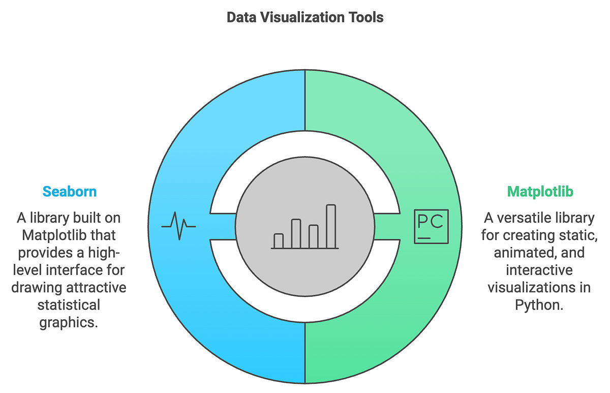
- Matplotlib: The foundational plotting library in Python. It's powerful and highly customizable, but can sometimes require a lot of code for complex plots.
- Seaborn: A high-level library built on top of Matplotlib. It's designed for creating beautiful and informative statistical graphics with much less code.
Let's get started by setting up our environment and diving into the most common types of plots.
1. Setting Up and a First Look at Distributions
Whenever you start a data visualization task, you'll typically import the same set of libraries.
Exploratory Data Analysis with Pandas Python
First, let's see the standard setup for a data analysis session in Python. The video 'Exploratory Data Analysis with Pandas Python' by Rob Mulla begins with this exact step.
Watch from 01:01 to 02:24. Pay attention to the conventional aliases used: pd for Pandas, np for NumPy, plt for Matplotlib's pyplot module, and sns for Seaborn. The plt.style.use('ggplot') is a common choice for aesthetically pleasing plots.
Now that we're set up, the first step in EDA is often univariate analysis—examining one variable at a time to understand its characteristics.
Histograms and Kernel Density Estimates (KDE)
For numerical variables, the most common way to view their distribution is with a histogram or a Kernel Density Estimate (KDE) plot.
- A histogram groups numbers into bins (or buckets) and shows the frequency of data points in each bin.
- A KDE plot can be thought of as a smoothed version of a histogram. Given your calculus background, you can think of it as an estimate of the variable's probability density function.
Let's watch a practical demonstration.
Exploratory Data Analysis with Pandas Python
The video 'Exploratory Data Analysis with Pandas Python' demonstrates how to create these plots to understand the distribution of a 'speed' feature in a dataset of roller coasters.
Watch from 20:57 to 27:29. Notice how a histogram quickly reveals the shape of the data, its central tendency, and its spread. The video also shows how a KDE plot provides a smoother view of the same distribution.
Bar Plots and Count Plots
For categorical variables, we can't calculate a mean or median. Instead, we want to see the frequency of each category. A bar plot or count plot is perfect for this.
Seaborn Tutorial : Seaborn Full Course
Let's turn to the comprehensive 'Seaborn Tutorial' by Derek Banas to see how Seaborn makes this incredibly easy with the countplot function.
Watch from 18:38 to 19:40. You'll see how a single line of code sns.countplot(x='sex', data=tips_df) can instantly generate a plot showing the counts of males and females in the dataset.
2. Visualizing Relationships: Bivariate Analysis
Univariate analysis is useful, but the real insights often come from bivariate analysis—exploring the relationship between two variables. The type of plot you choose depends on the types of the two variables.
Numerical vs. Numerical: Scatter Plots
To explore the relationship between two numerical variables (e.g., height and weight, engine size and price), the scatter plot is your go-to tool. Each point on the plot represents one observation (or row) from your dataset.
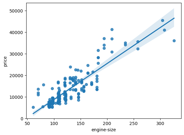
You can create scatter plots with Matplotlib, but Seaborn's scatterplot function adds useful features, like the ability to color points by a third, categorical variable using the hue parameter.
Exploratory Data Analysis with Pandas Python
Let's return to Rob Mulla's 'EDA with Pandas' video to see a comparison of creating scatter plots with Pandas/Matplotlib and then enhancing them with Seaborn.
Watch from 27:29 to 30:57. Observe how adding hue='year_introduced' to the Seaborn scatter plot adds a new layer of information, revealing how the relationship between speed and height has evolved over time.
Numerical vs. Categorical: Box Plots and Violin Plots
What if you want to compare a numerical variable across several categories? For instance, comparing the total bill amount for smokers vs. non-smokers, or for each day of the week. For this, box plots and violin plots are excellent.
- Box Plot: A concise summary of a variable's distribution. It shows the median (the center line), the interquartile range (IQR, the box), and the range of the data (the "whiskers"). Points outside the whiskers are potential outliers.
- Violin Plot: Combines a box plot with a KDE plot. It shows the same statistics as a box plot, but the width of the "violin" also shows the probability density of the data at different values.
Given your statistics knowledge, you should find the information presented in these plots very intuitive.
Seaborn Tutorial : Seaborn Full Course
The 'Seaborn Tutorial' provides a fantastic explanation of both plot types and what they represent.
Watch from 20:25 to 23:40. The video clearly breaks down the components of a box plot (median, quartiles, whiskers, outliers) and then introduces the violin plot as a richer alternative.
Correlation Heatmaps
When you have many numerical variables, you can compute a correlation matrix to see the pairwise correlation coefficient between every pair of variables. A heatmap is the perfect way to visualize this matrix. It uses color to represent values, making it easy to spot strong positive or negative correlations at a glance.
Seaborn Tutorial : Seaborn Full Course
Derek Banas demonstrates how to compute a correlation matrix and then visualize it with a heatmap in one simple step using Seaborn.
Watch from 32:55 to 35:25. He first creates a correlation matrix using df.corr() and then passes it to sns.heatmap(). The annot=True parameter is very useful for displaying the correlation values on the plot.
Test your understanding!
You have a dataset of house sales with the following columns: price (numerical), square_footage (numerical), and neighborhood (categorical). Which plot type would you use for each of the following questions?
- How is the
priceof houses distributed? - What is the relationship between
priceandsquare_footage? - How does the
pricecompare across differentneighborhoods?
Show answer
- A histogram or KDE plot of the
pricecolumn would be best to see its distribution. - A scatter plot with
square_footageon the x-axis andpriceon the y-axis would show the relationship between these two numerical variables. - A box plot or violin plot would be ideal. You would put
neighborhoodon the x-axis andpriceon the y-axis to compare the distribution of prices for each neighborhood.
3. High-Level Views with Seaborn
Seaborn's true power lies in its ability to create complex, multi-plot visualizations with a single function call. These are fantastic for getting a quick, high-level overview of your entire dataset.
Pair Plots
A pair plot (pairplot in Seaborn) creates a grid of plots showing the relationship between every pair of numerical variables in your DataFrame. It places scatter plots on the off-diagonals and histograms or KDE plots on the diagonal. It's one of the most useful commands in all of EDA.
Seaborn Tutorial : Seaborn Full Course
Let's see the pairplot in action. It's a powerful way to spot interesting relationships that you might want to investigate further.
Watch from 08:35 to 11:20. Notice how this single function gives you a comprehensive overview of the numerical columns. The video also shows how you can use hue to add a categorical dimension, which is extremely powerful.
Regression and Faceted Plots
Sometimes you want to see a scatter plot, but with a linear regression line fitted to the data to make the trend clearer. Seaborn's lmplot function does exactly this.
Even better, lmplot allows for faceting—creating a grid of plots where each plot shows a different subset of your data. You can specify which variable to use for the columns (col) and rows (row) of your plot grid.
Seaborn Tutorial : Seaborn Full Course
The final section of the 'Seaborn Tutorial' covers lmplot and demonstrates this faceting capability, which is a hallmark of advanced data visualization.
Watch from 54:43 to 59:33. The first part shows a basic lmplot. The key part is at 58:10, where he uses col='sex' and row='time' to create four separate plots, each showing the relationship between bill and tip for a specific combination of gender and time of day. This is an incredibly efficient way to explore interactions between variables.
Conclusion
Congratulations on completing the first module of our course! Today, you've learned how to bridge the gap between raw, clean data and genuine insight using visualization. This is not just about making pretty pictures; it's a fundamental part of the scientific process of building AI models.
Key Takeaways:
- Matplotlib is the foundational library, while Seaborn provides a high-level interface for creating beautiful statistical plots with less code.
- Univariate plots (histograms, KDEs, count plots) help you understand the distribution of single variables.
- Bivariate plots help you explore relationships between two variables. The choice of plot depends on the data types (scatter for num-num, box/violin for num-cat).
- Heatmaps are ideal for visualizing correlation matrices.
- High-level Seaborn functions like
pairplotandlmplotwith faceting allow for rapid, comprehensive exploration of your entire dataset.
This lesson concludes our work on Python and data science foundations. You are now equipped with the essential skills to load, manipulate, clean, and visualize data. These are the practical prerequisites for everything that follows.
In our next module, "Applied Linear Algebra for AI," we will begin our journey into the mathematical core of artificial intelligence. We'll start by exploring how vectors and matrices are used to represent data and perform linear transformations, a concept that underpins nearly every modern machine learning algorithm.