Welcome back. In our previous lessons, we successfully established a complete rendering pipeline, from creating a native window with SDL to setting up a GPU-accelerated Skia SkSurface to draw on. We now have a blank canvas, but the application itself is static. It's time to build the engine that will drive it forward.
This lesson tackles a fundamental concept in real-time applications: the application loop. Your goal is to structure a high-performance loop that separates application state updates from rendering. This architecture is critical for creating a fluid, responsive experience in your whiteboard application, ensuring that user interactions feel immediate and animations are smooth, regardless of the complexity of the scene or the performance of the user's hardware. This concept lies at the heart of systems programming for interactive software, from high-frequency trading platforms to the high-performance graphics application you are building.
The Challenge of Time in Interactive Applications
A naive application loop might try to update the application state and draw the screen in every single cycle. However, the time it takes to complete one cycle (a "frame") can vary dramatically based on the hardware and the current workload. If your application's logic is tied to this variable frame rate, its speed will be inconsistent—running too fast on powerful machines and grinding to a halt on slower ones.
This inconsistency is unacceptable for a high-quality user experience and can introduce subtle but critical bugs in physics and state management. The solution is to decouple the "simulation" time from "wall-clock" time.
The following video provides an excellent visual overview of this problem and introduces the architecture we will be implementing.
This short, animated video by Vittorio Romeo clearly explains the evolution from a simple, flawed game loop to the robust, fixed-timestep model.
Please watch the following segments: First, watch from the beginning until this point. This covers the basic loop, the introduction of a variable "delta time" to solve the speed issue, and the serious problems that this variable approach introduces, such as non-determinism and instability. Next, watch from this segment. This presents the solution: a loop that updates the simulation at a fixed frequency while rendering can happen at a variable rate. Pay close attention to the concepts of a "tick rate" and an "accumulator."
The Fixed Timestep, Variable Render Loop
As the video demonstrated, the superior architecture involves two distinct cadences:
- Update: The application state (e.g., stroke positions, camera physics, animations) is advanced in discrete, fixed-size time steps. For example, you might decide your simulation will always advance by 1/120th of a second per update. This ensures your application's logic is deterministic and stable.
- Render: The current state is drawn to the screen. This can happen as frequently as possible, independent of the update steps. A fast machine might render multiple times between updates, while a slow machine might skip rendering some frames to allow the update logic to catch up.
The key to managing this is an "accumulator" variable. In each iteration of the main loop, we measure the real time that has passed. This time is added to the accumulator. Then, we run the fixed-step update() function in a loop until the accumulator is less than the size of one fixed step.
For a deep and comprehensive explanation of this pattern, the "Game Loop" chapter from Robert Nystrom's book Game Programming Patterns is an invaluable resource.
Game Loop · Sequencing Patterns
This text provides one of the clearest explanations available for the fixed-timestep game loop pattern.
Please read the section titled Play catch up. Focus on understanding the lag variable (which we are calling the accumulator) and how the inner while loop ensures the game logic "catches up" to real time in fixed increments.
The resulting architecture is beautifully illustrated by this timeline from the article:

A Practical C++ Implementation
Let's translate this concept into a practical C++ implementation. The following video walks through adding a "semi-fixed timestep" (the same pattern we're discussing) to an existing C++ project. It provides a clear, step-by-step guide to the necessary code.
Advanced C++/Graphics Tutorial 29: Timestep!
This tutorial by "MakingGamesWithBen" is a great practical guide to implementing the loop structure in C++.
Watch the segment from this timestamp. It covers: Defining constants for desired FPS and frame time. Using SDL_GetTicks to measure elapsed time. Calculating a totalDeltaTime to feed the accumulator. Implementing the while loop that processes physics steps. A crucial, practical consideration: limiting the number of physics steps per frame with maxPhysicsSteps to prevent the "spiral of death" on very slow machines, where the simulation takes longer than real-time and the application freezes trying to catch up.
Refining the Loop: Interpolation for Visual Smoothness
There's one final, subtle issue with this model. Because rendering is decoupled from updates, we will often be rendering at a point in time between two simulation steps. If we simply draw the state from the last completed update, fast-moving objects will appear to stutter.
The solution is interpolation. When we render, we still have a small amount of time left in our accumulator—this tells us how far we are into the next simulation step. We can use this value (typically between 0.0 and 1.0) to interpolate the object's visual position between its state in the previous update and its state in the current update.
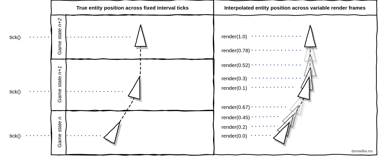
The "Game Programming Patterns" article also covers this refinement.
Game Loop · Sequencing Patterns
This section explains the final piece of the puzzle: smoothing out the visuals.
Now, please read the section titled Stuck in the middle. This explains why interpolation is necessary and how the lag variable provides the exact factor needed to perform it.
For a concrete code example, we can look at a well-regarded answer from the Game Development Stack Exchange. This answer provides a complete, working C++ implementation based on the famous "Fix Your Timestep!" article by Glenn Fiedler. While it uses a specific physics integration method (RK4), the overall loop structure and the interpolate function are universally applicable.
How to achieve smooth movement with a fixed timestep
This code provides a full reference for a fixed-timestep loop with interpolation.
Read through the code in the second answer. You don't need to understand the details of the integrate function (which implements RK4 physics). Instead, focus on these key parts: The applyPhysics function: Notice the while (accumulator>=dt) loop, which is the core of our pattern. The interpolate function: See how it takes the previous state, the current state, and an alpha value (calculated from accumulator/dt) to produce a blended State for rendering. The final line in applyPhysics: pPlayerSprite->setPosition(state.statePosition);, where this interpolated state is used to set the visual position of the sprite. This is the final connection between our simulation and what the user sees.
Conclusion
In this lesson, you've learned how to architect a robust, high-performance application loop that is essential for any real-time interactive software. By decoupling state updates from rendering, you gain determinism, stability, and consistent performance across a wide range of hardware.
Key Takeaways:
- Tying application logic directly to the frame rate leads to inconsistent behavior and instability.
- The standard high-performance solution is a loop with fixed-timestep updates and variable-rate rendering.
- An accumulator variable tracks elapsed real time, and a
whileloop processes a series of fixed-step updates to "catch up." - To prevent visual stuttering, interpolation between the last two simulation states should be used for rendering, creating the illusion of perfectly smooth motion.
- Practical limits, like capping the number of updates per frame, are necessary to prevent the "spiral of death" on systems under heavy load.
You now have the complete architectural foundation for your application. The windowing and graphics backend are initialized, and a powerful main loop is ready to drive them. In our next lesson, we will finally begin drawing on our canvas, starting with Skia's SkPaint object to control the color, style, and thickness of shapes.