Interpreting SLR Coefficients

In our previous lesson, we focused on navigating R's regression output to quickly locate key numbers. You now have a mental map for finding the coefficient estimates in the summary() output. Today, we shift from locating to interpreting. Our goal is to understand what the intercept ( $β^_{0}$ ) and slope ( $β^_{1}$ ) coefficients truly mean in a simple linear regression model and, crucially, how to articulate that meaning in a way that will satisfy your professor.

This lesson is foundational for almost every exam question you'll face. We will break down the precise, exam-style sentences you need to interpret each coefficient, paying special attention to common traps like misinterpreting the intercept and confusing association with causation.

The Building Blocks: Intercept and Slope

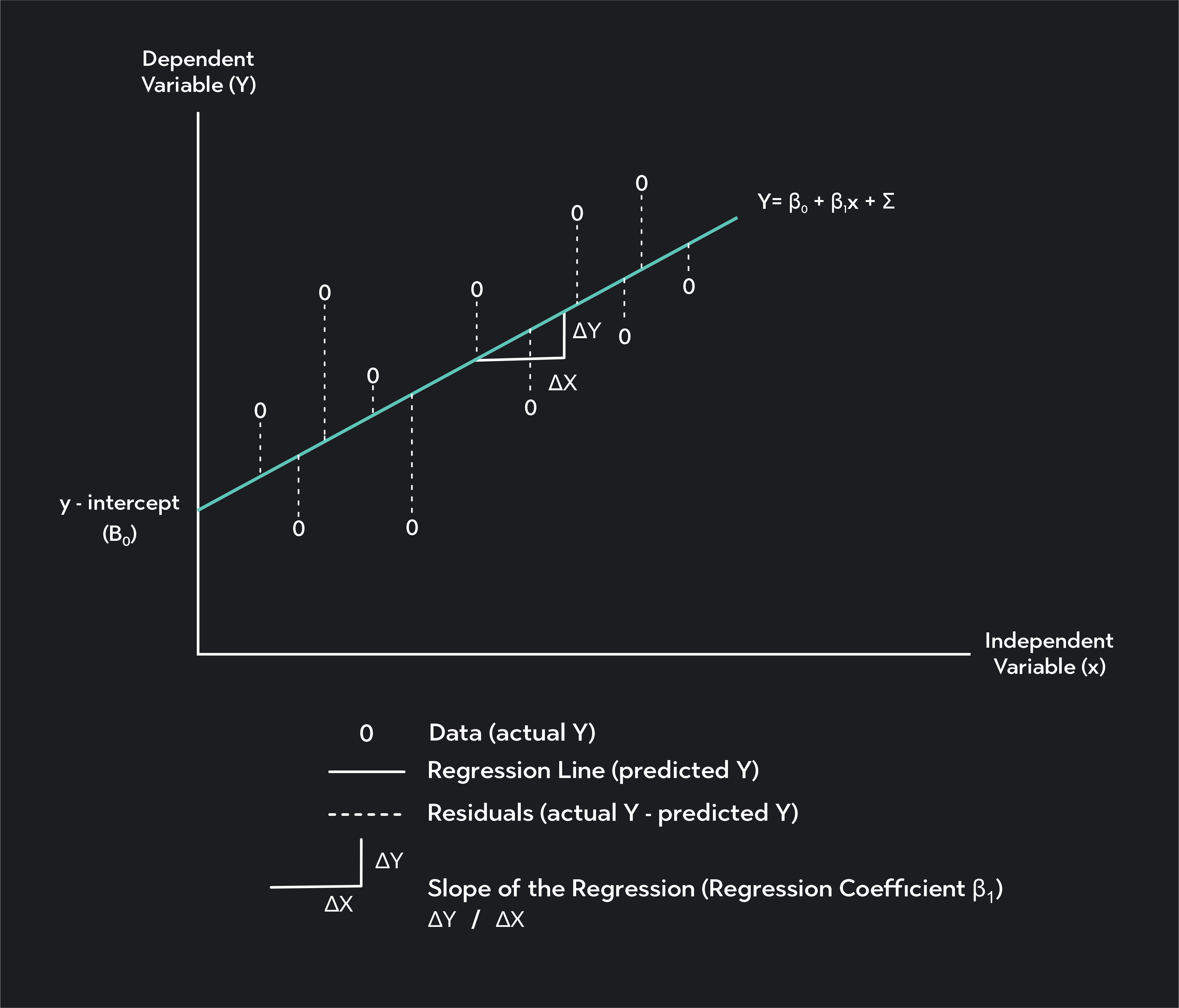
In simple linear regression, we model the relationship between two variables using a straight line. The equation for this line is:

Y^= β^_{0} + β^_{1} X

Here:

$Y^$ (Y-hat) is the predicted value of the dependent variable.
$X$ is the independent (or predictor) variable.
$β^_{0}$ is the estimated Y-intercept, the point where the line crosses the Y-axis.
$β^_{1}$ is the estimated slope of the line.

The image below provides a clear visual breakdown of these components.

This diagram illustrates the key elements of a simple linear regression model. The Y-intercept ($\beta_0$) is where the regression line meets the vertical axis, and the slope ($\beta_1$) represents the line's steepness ($\Delta Y / \Delta X$).

Now, let's learn the formal interpretation of these parameters. The following video provides an excellent conceptual overview.

Simple Linear Regression: Interpreting Model Parameters

This video from jbstatistics clearly explains the theoretical meaning of the intercept and slope parameters and their sample estimates. It also introduces two critical nuances you must be aware of for your exam: the problem of extrapolation and the difference between association and causation.

Please watch these key segments: The Intercept (β₀): Focus on the definition: the mean of Y when X is zero, and the important warning about this being a "massive extrapolation" if X=0 is outside your data range. The Slope (β₁): Understand this as the change in the mean of Y for a one-unit increase in X. Note the crucial distinction made here between association and a causal link. Intercept Example: See how the interpretation of the intercept can be nonsensical in a real-world context (a fish with zero length). This is a classic exam point. Slope Example: This provides a template for a precise interpretation of the slope estimate in context.

From Theory to Exam-Ready Interpretation

The video gave you the concepts. Now, let's translate them into the kind of direct, practical answers required for your exam, using a real R output.

Interpreting the Intercept ( $β^_{0}$ )

What to look for: The Estimate value for the (Intercept) row in the Coefficients table.

How to Interpret (The Template):
"The predicted value of [Dependent Variable Y] is [ $β^_{0}$ value] when the [Independent Variable X] is 0."

Common Trap: Always ask yourself: "Does X=0 make practical sense?"

If yes (e.g., advertising budget = 0), the interpretation is meaningful.
If no (e.g., height = 0, weight = 0), the intercept is often just a mathematical necessity to anchor the line and may not have a useful real-world interpretation. Acknowledging this shows a deeper understanding.

Interpreting the Slope ( $β^_{1}$ )

What to look for: The Estimate value for your predictor variable's row in the Coefficients table.

How to Interpret (The Template):
"For each one-[unit] increase in [Independent Variable X], the predicted value of [Dependent Variable Y] is expected to [increase/decrease] by [ $β^_{1}$ value] [Y-units]."

Common Trap (CRITICAL): Association is not causation. Your professor is strict about this. Never say "an increase in X causes an increase in Y." Regression on observational data only describes a relationship.

To avoid this trap, use precise, non-causal language. The following reading provides an excellent example of how to phrase your interpretation carefully.

4.3 SLR model with a continuous predictor | Introduction to Regression Methods for Public Health Using R

This resource shows how to report regression results professionally. We will focus on the phrasing used, which is perfect for avoiding causal claims.

Find the subsection "4.3.3 Writing it up". Read the example interpretation sentence: this one. Notice the wording: "...for every 1-cm difference in waist circumference, adults differ in mean fasting glucose..." This phrasing is excellent because it describes an observed association in the data without implying that changing one variable will cause a change in the other. Adopting this style will be very effective for your exam.

Practice Drill

Let's apply this with an exam-style question. The output below models sales revenue as a function of the number of ads run.

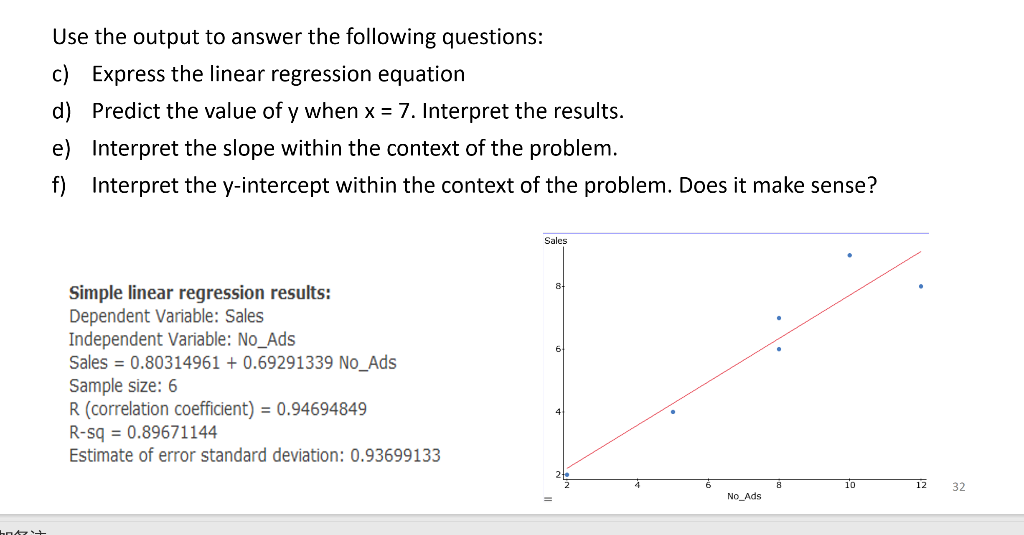
This output shows the results of a simple linear regression. The dependent variable is 'Sales' and the independent variable is 'No_Ads'. We will use this to practice interpreting the coefficients.

Using the output, answer the following questions.

Your Task:

Interpret the slope within the context of the problem.
Interpret the y-intercept within the context of the problem. Does it make sense?

Solutions

Here are model answers in the precise, 2-line format your professor will be looking for.

Slope Interpretation:
- Answer: For each additional ad that is run, the predicted sales are expected to increase by 0.6929. Since the variables are not given units, we state it generally. If sales were in thousands of dollars, we would say "$692.90".
- Alternative (using the non-causal language): On average, a 1-unit difference in the number of ads is associated with a 0.6929 unit difference in mean sales.
Y-Intercept Interpretation:
- Answer: When the number of ads is zero, the predicted sales are 0.8031.
- Does it make sense? Yes, this interpretation is plausible. It could represent a baseline level of sales that occurs even with no advertising, perhaps through word-of-mouth or existing brand recognition.

Conclusion

In this lesson, we moved from identifying coefficients to interpreting them. You now have a clear framework and precise templates for explaining the meaning of the intercept ( $β^_{0}$ ) and the slope ( $β^_{1}$ ) in a simple linear regression model.

The key takeaways are:

Intercept ( $β^_{0}$ ): The predicted value of Y when X is 0. Always question if X=0 is a practical or meaningful value.
Slope ( $β^_{1}$ ): The predicted change in Y for a one-unit change in X.
The Golden Rule: Always use non-causal language ("is associated with," "is expected to change by," "differs by") unless you are working with data from a controlled experiment.

We've interpreted the coefficients individually. In the next lesson, we'll combine them to interpret the full regression equation as a whole, another common exam task.

Recommended resources