With this lesson, we conclude our module on diagnosing the assumptions of linear regression. In the previous lessons, you learned to use residual plots to check for linearity and homoscedasticity, and the Normal Q-Q plot to assess the normality of residuals. Now, we'll tackle the fourth and final pillar: the independence of residuals.
This assumption states that the error term for any single observation is not correlated with the error term of any other observation. While always a requirement, it becomes a primary concern when dealing with data collected over time, such as daily stock prices or monthly sales figures. Violation of this assumption is called autocorrelation or serial correlation.
Today's lesson will equip you to explain the independence assumption and, crucially, to detect its violation. We will cover visual detection using residual plots and formal testing with the common Durbin-Watson test. This is the last step in ensuring your model's foundation is sound before we move on to interpreting more complex models.
The Independence Assumption and Autocorrelation
The independence assumption is critical for the reliability of our hypothesis tests. When it's violated, our standard errors for the coefficients become biased, which in turn makes our t-statistics, p-values, and confidence intervals untrustworthy. While the coefficient estimates themselves remain unbiased, our ability to make valid inferences about them is compromised.
The following reading clearly defines autocorrelation and its consequences.
14.5 Autocorrelation Tests | A Guide on Data Analysis - Bookdown
This guide provides a concise and practical overview of autocorrelation.
Read the introductory paragraphs, starting from the definition down to the list of its consequences. Pay close attention to the impact on standard errors and hypothesis tests, as this is a key exam point.
Autocorrelation means the residuals are not random; they contain a pattern. For a quick visual introduction to this concept, the following video segment is very helpful.
Assumptions in Linear Regression - explained | residual analysis
This video from TileStats provides a clear, animated explanation of the core regression assumptions.
Watch the short segment on the independence assumption, from the introduction. It effectively visualizes what a pattern in residuals over time looks like and introduces the Durbin-Watson test, which we will cover next.
Visual Detection: The Residuals vs. Order Plot
Our first line of defense is, as always, a plot. For autocorrelation, we use a residuals vs. order plot. The y-axis shows the residuals, and the x-axis shows the order in which the data were collected (e.g., time 1, 2, 3...).
Important: This plot is only meaningful if your data has a natural sequence. For a random sample of people surveyed at the same time, this plot is irrelevant.
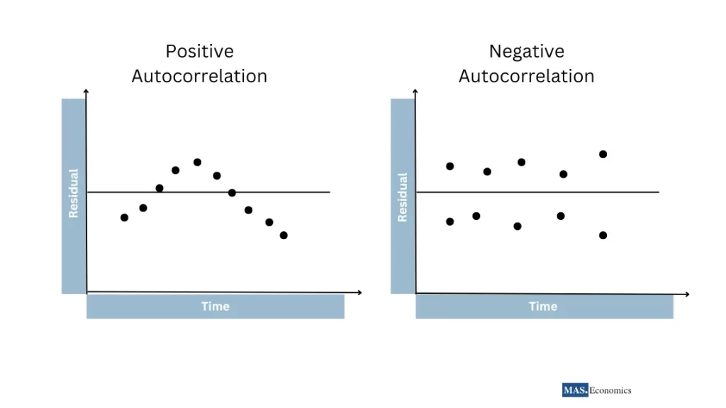
- No Autocorrelation (Good!): The residuals will appear as a random scatter of points around the zero line. There is no discernible pattern.
- Positive Autocorrelation: Residuals of the same sign will tend to cluster together. You'll see runs of positive residuals followed by runs of negative residuals, often creating a wave-like or cyclical pattern.
- Negative Autocorrelation: Residuals will tend to alternate signs. A positive residual is likely to be followed by a negative one, and vice-versa, creating a zig-zag pattern.
The images below illustrate these patterns clearly.
For a more detailed walkthrough of these plots, the following resource is excellent.
4.5 - Residuals vs. Order Plot | STAT 501
This page from Penn State's STAT 501 course gives clear examples of what to look for in a residuals vs. order plot.
First, read the introduction to understand the plot's purpose and the critical condition for its use: the main prerequisite. Then, review the examples for positive serial correlation and negative serial correlation.
Formal Detection: The Durbin-Watson Test
While visual inspection is useful, your exam will require you to interpret a formal statistical test. The most common test for first-order autocorrelation is the Durbin-Watson (DW) test.
Hypotheses:
- Null Hypothesis (H₀): There is no first-order autocorrelation (the autocorrelation coefficient, ρ, is 0).
- Alternative Hypothesis (H₁): There is first-order autocorrelation (ρ ≠ 0).
The DW Statistic:
The test produces a statistic, , that ranges from 0 to 4.
- : Indicates no autocorrelation.
- (approaching 0): Suggests positive autocorrelation.
- (approaching 4): Suggests negative autocorrelation.
The Decision Rule:
Historically, decisions were made by comparing the DW statistic to two critical values, a lower bound () and an upper bound (), which created "inconclusive" regions.
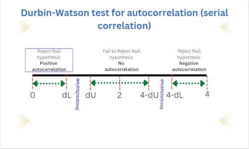
In modern software, including R, the interpretation is much simpler: you just use the p-value.
Let's see how this works with an R output.
14.5 Autocorrelation Tests | A Guide on Data Analysis - Bookdown
This part of the guide shows the R code and output for the Durbin-Watson test.
Focus on the sections 1. Durbin-Watson Test and Interpretation of the Results. First, look at the R output for dwtest(model). You will see the key values: the DW statistic and the p-value. Then, read the corresponding interpretation section. For your exam, the p-value approach is the most direct: if p < 0.05, you reject H₀.
In the example from the reading, the DW statistic is 0.77291. This is much less than 2, strongly suggesting positive autocorrelation. The p-value is extremely small (3.323e-10), confirming this. We would confidently reject the null hypothesis.
For a deeper dive into the logic of the DW test and its causes, the following video is exceptional.
What is autocorrelation? Extensive video!
The "zedstatistics" channel offers a very thorough explanation of autocorrelation.
First, watch the section on the consequences of autocorrelation from this timestamp. It clearly explains why this assumption matters for your standard errors and p-values. Next, watch the detailed explanation of the Durbin-Watson test from this timestamp. The presenter does an excellent job of explaining the logic behind the test statistic and the decision regions.
Broader Context: Other Tests
For your exam, the Durbin-Watson test is the most important one to know for autocorrelation. However, it's good to be aware that it primarily tests for first-order correlation (i.e., between adjacent residuals). A more general test, which can handle higher-order autocorrelation, is the Breusch-Godfrey (BG) test. It also uses a p-value for its decision rule. You don't need to know the details, but knowing its name and purpose demonstrates a wider understanding.
Exam-Style Interpretation
Here is how you frame your conclusions for the exam:
-
From a Plot:
The residuals vs. order plot shows a clear cyclical pattern, with clusters of positive and negative residuals. This visual evidence suggests the presence of positive autocorrelation, violating the independence assumption.
-
From a Durbin-Watson Test:
The Durbin-Watson test yielded a statistic of DW = 0.77 with a p-value < 0.05. Since the DW statistic is significantly less than 2 and the p-value is below the 0.05 significance level, we reject the null hypothesis and conclude that there is significant positive first-order autocorrelation in the residuals.
Practice Drill
You are analyzing monthly sales data for a company and produce the following output after running a regression.
R Output:
Durbin-Watson test

data:  sales_model
DW = 2.89, p-value = 0.002
alternative hypothesis: true autocorrelation is greater than 0
(Note: Some software may test a one-sided alternative. A two-sided test is more general. Given the DW of 2.89, we suspect negative autocorrelation. The small p-value strongly suggests we reject the null of no autocorrelation anyway.)
Residuals vs. Order Plot:
The plot shows a distinct zig-zag pattern, with most positive residuals being followed by negative residuals and vice-versa.
Your Task:
Write a 2-3 sentence, exam-style conclusion about the independence assumption for this model.
Solution
Exam-Style Conclusion:
The residuals vs. order plot shows a distinct alternating pattern, suggesting negative autocorrelation. This is confirmed by the Durbin-Watson test, which gives a statistic of 2.89 (p=0.002). Since the DW value is significantly greater than 2 and the p-value is less than 0.05, we reject the null hypothesis of no autocorrelation and conclude the independence assumption is violated due to significant negative serial correlation.
Conclusion
Congratulations, you have now completed your diagnostic toolkit for linear regression! You are equipped to check all four major assumptions: Linearity, Independence, Normality, and Homoscedasticity (L.I.N.E.).
Key Takeaways:
- The independence assumption states that error terms are uncorrelated with each other. Violation is called autocorrelation.
- Autocorrelation is most common in time-series data.
- It is detected visually with a residuals vs. order plot, looking for non-random patterns (waves for positive, zig-zags for negative).
- It is detected formally with the Durbin-Watson test. A statistic near 2 means no autocorrelation, while values approaching 0 (positive) or 4 (negative) indicate a violation. A small p-value (< 0.05) confirms this.
With model diagnostics covered, we are now ready to move on. In the next module, we will focus on interpreting models with multiple predictors, including categorical variables, and how to handle their complexities.