Interpreting Individual Slopes in MLR

From a Line to a Plane: Visualizing MLR

In simple linear regression, we modeled the relationship between two variables, which we could visualize as a line on a 2D scatter plot. The slope of that line was unambiguous.

In multiple regression, we are modeling the relationship between a response variable $Y$ and multiple predictor variables $X_1,X_2,\dots ,X_p$. With two predictors, our model is no longer a line, but a plane slicing through a 3D cloud of data points.

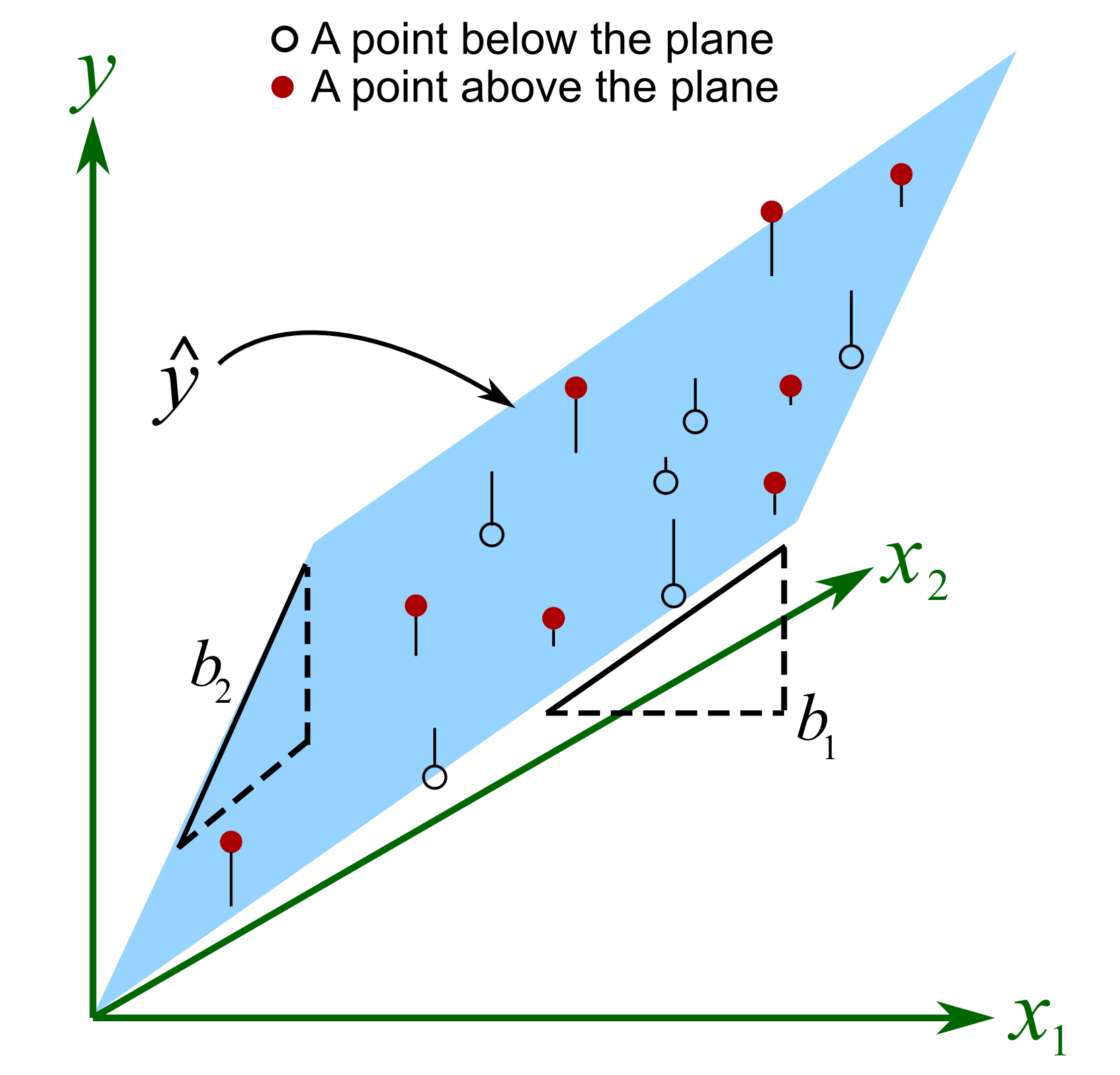
The equation for this model is an extension of the SLR equation:

The key question is: what does $b_1$ mean now that $b_2,\dots ,b_p$ are also in the model? The coefficient $b_1$ represents the slope of the plane in the direction of the $X_1$ axis. To measure this, you must move along the $X_1$ axis while your position on the $X_2$ axis is held fixed. This is the geometric intuition behind the core concept of MLR interpretation.

The Golden Rule of MLR Interpretation

The most common mistake in interpreting MLR is to treat a coefficient like a simple slope. The presence of other variables in the model fundamentally changes the interpretation.

As the reading makes clear, the interpretation of any single coefficient ${\beta }_j$ is conditional on the other predictors in the model. This leads us to our exam-style template.

Exam-Style Sentence Template:

A one-unit increase in [Predictor Variable $X_j$] is associated with a [$b_j$]-unit [increase/decrease] in the predicted [Response Variable $Y$], holding all other variables in the model constant.

Notice the use of "is associated with." This is a crucial distinction. Unless you have performed a rigorous causal analysis (which is beyond the scope of a standard regression model), you are describing a conditional association, not a causal relationship. Using "causes" or "leads to" is a common exam trap that you must avoid.

This short video provides an excellent summary of this rule and why the wording is so important.

Why "Holding Others Constant" Changes Everything

This isn't just a phrase to memorize; it reflects a fundamental property of MLR. A variable's estimated effect can change dramatically—even reversing its sign—when other predictors are added to the model.

Let's consider a classic example: predicting house price.

• Model 1 (SLR): Price ~ Bedrooms. In this model, you would likely find a positive coefficient. An extra bedroom is associated with a higher price.
• Model 2 (MLR): Price ~ Bedrooms + Square_Footage. Here, you might find that the coefficient for Bedrooms becomes negative. Why? The model is now telling you the effect of adding a bedroom while holding square footage constant. Adding a bedroom to a house of a fixed size means all the rooms (including the new bedroom) must be smaller, which could be less desirable and thus associated with a lower price.

The coefficient for Bedrooms in Model 1 and Model 2 are measuring different things. The first measures the simple association, while the second measures the association conditional on the house size.

The following reading demonstrates this exact phenomenon with R output.

From Theory to Practice: Interpreting R Output

Let's apply this to a full example. The following reading analyzes data on literacy rates, newspaper circulation, and radio/TV ownership.

Let's use the output from that reading to interpret the coefficient for radios.

Output Snippet:

Predictor         Coef
...
radios       -0.0003535
...

Variable Definitions:

• Response: Literacy rate (proportion)
• Predictors: newspaper copies, radios, television sets (all measured as units per 1000 people)

Your Task: Using our template, how would you interpret the coefficient for radios?

Practice Drill

You are given the following partial R output for a model predicting house price (in thousands of dollars).

Coefficients:
            Estimate
(Intercept) 565.300
House_Size    0.113  (in square feet)
Distance    -15.975  (in miles from city center)
Age           0.285  (in years)

Your Task:

1. Write a precise, exam-style sentence interpreting the coefficient for House_Size.
2. Write a precise, exam-style sentence interpreting the coefficient for Distance.

Conclusion

This lesson introduced the single most important rule for interpreting coefficients in multiple linear regression. You learned that the effect of any one predictor is conditional on the other variables included in the model.

Key Takeaways:

• The interpretation of a coefficient ${\beta }_j$ in MLR is the expected change in $Y$ for a one-unit change in $X_j$, holding all other predictor variables constant.
• This "holding constant" clause is not optional; a variable's coefficient can change in both magnitude and sign when other variables are added or removed.
• For your exam, always use the phrase "is associated with" rather than "causes" to describe the relationship. The template is your friend: A 1-unit change in X is associated with a B-unit change in Y, holding Z constant.

So far, we have only interpreted the value of the coefficients. We have not yet discussed whether these values are statistically meaningful or if they could have occurred by random chance. In the next lesson, we will do just that by learning to assess the statistical significance of individual predictors using their t-statistics and p-values.