T-tests and p-values for MLR Predictors

In the previous lesson, you mastered the crucial art of interpreting the value of a coefficient in a multiple linear regression model, always remembering to add the phrase "holding all other variables constant." Now, we'll answer the next logical question your examiner will have: is that coefficient's effect real, or could it just be due to random chance?

This lesson focuses on assessing the statistical significance of individual predictors. You will learn to use the t-statistics and p-values from a regression output to confidently determine whether a variable has a meaningful linear relationship with the response. This skill is fundamental for building and refining a model, and for correctly interpreting any output you're given on the exam.

Is the Relationship Real? The Hypothesis Test for a Coefficient

When a model estimates a coefficient, say $b_{1} = 0.5$ , it's just an estimate from our sample data. The true value in the entire population, $β_{1}$ , might be different. Specifically, we want to know if it could plausibly be zero. If $β_{1}$ is zero, it means there's no actual linear relationship between that predictor and the response variable, after accounting for the other variables in the model.

This leads to a formal hypothesis test for each coefficient $β_{j}$ :

Null Hypothesis ( $H_{0}$ ): $β_{j} = 0$ . (The predictor $X_{j}$ has no linear effect on $Y$ , holding other variables constant.)
Alternative Hypothesis ( $H_{1}$ ): $β_{j} \neq = 0$ . (The predictor $X_{j}$ has a statistically significant linear effect on $Y$ , holding other variables constant.)

To make this decision, we look at two key columns in the R output: the t value and the Pr(>|t|).

Decoding the R Output: t-values and p-values

Let's look at a standard regression output. The Coefficients table is your main focus here.

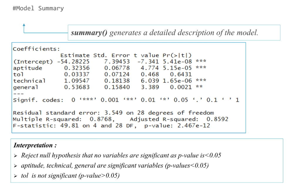
This R `summary()` output shows the Coefficients table. For each predictor, it lists the Estimate, Std. Error, t value, and p-value (`Pr(>|t|)`).

Here’s what each part tells you:

Estimate: The value of the coefficient ( $b_{j}$ ), which you learned to interpret in the last lesson.
Std. Error: A measure of the uncertainty or variability of the Estimate. A smaller standard error means a more precise estimate.
t value: This is the Estimate divided by its Std. Error. It tells you how many standard errors the coefficient is away from zero. A large absolute t-value suggests the coefficient is unlikely to be zero. A common rule of thumb for exams is that an absolute t-value greater than 2 is a strong indicator of significance.
Pr(>|t|): This is the p-value. It's the most direct tool for your decision. It represents the probability of observing an effect as large as you did if the null hypothesis (that the true effect is zero) were true.

The following short video provides an excellent walkthrough of how to conduct this hypothesis test for each coefficient using a typical regression output.

Multiple Regression | Coefficients – Interpretation, C.I, Hypothesis Testing

This video from Joshua Emmanuel clearly explains the process of testing the significance of each coefficient.

Watch the section on testing significance. Pay close attention to how the null/alternative hypotheses are stated and how the p-value is used to make a decision to reject or fail to reject the null hypothesis.

The Decision Rule: Your Exam-Day Shortcut

For your practical exam, the decision process is straightforward and relies on the p-value:

If p-value < 0.05, reject $H_{0}$ . Conclude the predictor is statistically significant.
If p-value ≥ 0.05, fail to reject $H_{0}$ . Conclude the predictor is not statistically significant.

The resource below gives a clear, text-based explanation of this rule and shows how to apply it to an R output, distinguishing between significant and non-significant predictors.

Multiple linear regression made simple

This article from Stats and R provides another example of interpreting a full regression output.

In the section "Interpretations of coefficients," focus on the part where the author interprets the Coefficients table. Read through the bullet points that explain how to conclude whether each variable is significant based on its p-value. Notice how they handle both significant and non-significant results.

Putting It All Together: Crafting the Perfect Exam Answer

Now, let's combine what you learned in the last lesson with today's topic. A complete answer involves interpreting both the coefficient's value and its significance.

The following reading provides excellent, exam-ready sentences that do exactly this.

Chapter 40 Estimating Incremental Validity of a Selection Tool Using Multiple Linear Regression | R for HR: An Introduction to Human Resource Analytics Using R

This article from "R for HR" demonstrates how to write up regression results with professional precision.

Find the section "Interpret Multiple Linear Regression Model Results" and read the paragraph interpreting the coefficients for SJT and Interview. Focus on the two-part sentences that first state the interpretation of the coefficient value and then state the conclusion about statistical significance, like this one: SJT interpretation. This is the structure you should aim for.

Let's apply this to our Model Summary image.

Example 1: The technical predictor

Estimate: 1.09547
p-value: 1.65e-06 (which is 0.00000165)

Exam-Style Answer:

A one-unit increase in the technical score is associated with a 1.095-point increase in the predicted response, holding all other variables constant. This relationship is statistically significant as its p-value (p < 0.001) is less than 0.05.

Example 2: The tol predictor

Estimate: 0.03337
p-value: 0.468

Exam-Style Answer:

The p-value for the tol predictor is 0.468, which is greater than 0.05. Therefore, there is not enough evidence to conclude that tol is a statistically significant predictor of the response variable, after controlling for the other predictors in the model.

Common Exam Trap: Do not interpret the magnitude of a non-significant coefficient. If a variable is not significant, its estimated effect is statistically indistinguishable from zero. Your interpretation should stop at stating it is not significant.

Practice Drill

You are given the following R output for a model predicting employee job_satisfaction (on a 1-100 scale) based on their tenure (in years), salary (in thousands of dollars), and team_size.

Coefficients:
            Estimate Std. Error t value Pr(>|t|)
(Intercept)  25.500     5.100      5.000  1.2e-06 ***
tenure        2.100     0.700      3.000  0.003   **
salary        0.500     0.100      5.000  1.2e-06 ***
team_size    -0.200     0.250     -0.800  0.425

Your Task:

Identify which predictors are statistically significant at the $α = 0.05$ level.
Write a complete, two-part exam-style interpretation for the salary coefficient.
Write a complete exam-style interpretation for the team_size coefficient.

Solution

Significant Predictors:
- tenure is statistically significant because its p-value (0.003) is less than 0.05.
- salary is statistically significant because its p-value (1.2e-06) is less than 0.05.
Interpretation for salary:

For each additional thousand dollars in salary, predicted job satisfaction is associated with an increase of 0.5 points, holding tenure and team size constant. This relationship is statistically significant (p < 0.001).
Interpretation for team_size:

The p-value for team_size is 0.425, which is greater than 0.05. Therefore, we do not have sufficient evidence to conclude that team size is a statistically significant predictor of job satisfaction, after accounting for tenure and salary.

Conclusion

You have now added another essential layer to your interpretation skills. You can look at a regression output, identify the key predictors, and make a statistically-backed judgment about the reality of their effects.

Key Takeaways:

The significance of a predictor is tested using the null hypothesis $H_{0} : β_{j} = 0$ .
The p-value is your primary tool. If p < 0.05, the predictor is statistically significant.
The t-statistic gives you context; a large absolute value (typically > 2) also indicates significance.
A complete exam answer addresses both the magnitude of the coefficient ("a one-unit increase in X...") and its statistical significance ("...and this effect is statistically significant (p < 0.05)").

In the next lesson, we will continue exploring coefficients by looking at a special case: dummy variables. You'll learn how to interpret the results when your predictor isn't a continuous number but a category, like 'Yes' vs. 'No' or 'Group A' vs. 'Group B'.