Interpreting Dummy Variable Coefficients

Welcome to the next lesson in your high-intensity regression course. In our previous sessions, we focused on interpreting coefficients for continuous numerical predictors—like age or salary—and determining their statistical significance. You learned the critical importance of the phrase "holding all other variables constant."

Today, we address a different but equally common scenario: how to incorporate non-numerical, or categorical, variables into your regression model. What happens when your predictor is something like "Marital Status" (Single, Married, Divorced) or "Location" (Urban, Rural)? You can't multiply "Urban" by a coefficient. The solution is to use dummy variables. This lesson will teach you how to interpret the coefficients for these variables, which is a crucial skill for your exam as it allows you to compare different groups within your data.

From Categories to Numbers: What is a Dummy Variable?

Linear regression requires all predictor variables to be numbers. To include a categorical variable, we must convert its categories into a set of special numeric variables called dummy variables (or indicator variables).

A dummy variable is a binary variable that takes a value of 1 if a certain category is present for an observation and 0 if it is not.

The rule is simple: if you have a categorical variable with k levels (or categories), you will create k-1 dummy variables. The one category that does not get its own dummy variable is called the base category or reference level. All comparisons are made relative to this base.

Look at the image below. The 'Marital Status' variable has three categories: 'Single', 'Married', and 'Divorced'. To include it in a model, we create two (k-1 = 3-1 = 2) dummy variables: 'Married' and 'Divorced'.

This table shows how a categorical variable, 'Marital Status', is converted into two dummy variables. 'Single' is the reference category, indicated by having a 0 in both the 'Married' and 'Divorced' columns.

If an individual is 'Married', the Married dummy variable is 1 and Divorced is 0.
If an individual is 'Divorced', the Divorced dummy variable is 1 and Married is 0.
If an individual is 'Single' (the base category), both dummy variables are 0.

Interpreting the Coefficient of a Dummy Variable

So, what does the coefficient of a dummy variable tell us? It represents the predicted change in the response variable for an observation in that category, compared to the base category, holding all other variables in the model constant.

Essentially, the coefficient shows how much the intercept of the regression line shifts up or down for that specific group compared to the reference group.

Let's watch a short video that clearly explains this concept using a model predicting lung capacity from age and smoking status (smoker vs. non-smoker).

Including Variables/ Factors in Regression with R, Part I | R Tutorial 5.7 | MarinStatsLectures

This video from MarinStatsLectures provides a great, clear explanation of how a binary dummy variable works and how to interpret its coefficient.

First, watch the section showing how the regression equation is calculated for non-smokers and smokers. Notice how the dummy variable's coefficient is either included (for smokers) or not (for non-smokers). Then, pay close attention to the interpretation of the effect of smoking.

As the video explains, the coefficient for the smoke dummy variable (e.g., -0.649) is the estimated difference in mean lung capacity between a smoker and a non-smoker (the base category), for any given age.

Exam-Style Sentence Template:

When interpreting a binary dummy variable coefficient, your answer should look like this:

"The predicted [response variable] for [Category 1] is, on average, [coefficient value] units higher/lower than for [Base Category], holding all other variables constant."

Working with More Than Two Categories

The logic extends directly to variables with more than two categories. Each of the k-1 dummy variables will have a coefficient that compares its category directly to the base category.

This next reading provides excellent, precise interpretations for dummy variables in an R output. It examines the effect of being Black, living in the South, or an Urban area on monthly earnings.

Dummy Variables in Regression - James Murray

This tutorial by James Murray provides clear examples and interpretations of dummy variables in a regression context.

First, look at the R output presented in the section "Example: Factors Affecting Monthly Earnings" to see how the dummy variables (Black, South, Urban) appear in the coefficients table. Then, carefully read the section immediately following it, which provides three paragraphs of interpretation for each of the dummy variables. This is the exact style of explanation you should aim for.

The key takeaway is that the coefficient for Urban (174.63) means that urban dwellers are predicted to earn, on average, $174.63 more per month than non-urban dwellers (the base category), after accounting for all other variables like education, experience, and IQ.

Let's look at an R output that demonstrates how R often handles this automatically when you use a factor() variable.

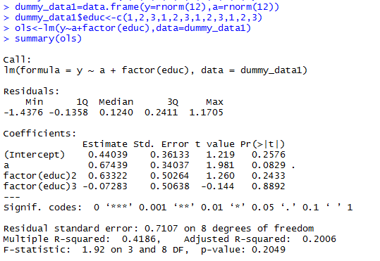
This R output shows a regression model where 'educ' is a categorical variable with three levels. R has automatically created two dummy variables: `factor(educ)2` and `factor(educ)3`. The base category is `educ=1`.

Here's how to interpret this output:

Reference Category: The category educ=1 is the reference level because it does not have its own row in the coefficient table.
factor(educ)2 coefficient (0.63322): The predicted response y for a person in education group 2 is, on average, 0.63322 units higher than for a person in education group 1, holding variable a constant.
factor(educ)3 coefficient (-0.07283): The predicted response y for a person in education group 3 is, on average, 0.07283 units lower than for a person in education group 1, holding variable a constant.

Common Exam Traps

Comparing Two Non-Reference Categories: In the example above, the coefficient for factor(educ)3 (-0.07283) compares group 3 to group 1. It does not compare group 3 to group 2. Your exam might trick you into making this mistake.
Misidentifying the Base Category: Always check which category is missing from the output table. That is your reference level. R often defaults to the first category numerically or alphabetically.
Forgetting "Holding Others Constant": This is as crucial for dummy variables as it is for continuous ones. The comparison is only valid after accounting for the influence of all other predictors in the model.

Practice Drill

You are given the R output from the reading "Dummy Variables in Regression," where the model predicts MonthlyEarnings.

Coefficients:
                Estimate Std. Error t value Pr(>|t|)    
(Intercept)     -475.254    143.374  -3.315 0.000968 ***
IQ                 3.169      1.223   2.590 0.009816 ** 
Knowledge          6.412      2.226   2.881 0.004097 ** 
YearsEdu          45.563      8.664   5.259 1.97e-07 ***
YearsExperience   13.356      3.969   3.365 0.000810 ***
Tenure             3.711      2.954   1.256 0.209459    
Black           -107.905     55.539  -1.943 0.052460 .  
South            -37.840     31.072  -1.218 0.223732    
Urban            174.627     31.904   5.474 6.29e-08 ***

The variables Black, South, and Urban are dummy variables where 1 indicates the person has that characteristic and 0 indicates they do not (the base category).

Your Task:

For the South dummy variable, what is the base/reference category?
Write a precise, exam-style sentence interpreting the coefficient for the YearsEdu variable. (This is a review from the previous lesson).
Write a precise, exam-style sentence interpreting the coefficient for the Urban variable. Make sure to state whether the effect is statistically significant at the $α = 0.05$ level.

Solution

Base Category for South: The base category is "non-Southern" or people who do not live in a Southern U.S. state.
Interpretation for YearsEdu:

For each additional year of education, the predicted monthly earnings are associated with an increase of $45.56, holding all other variables constant.
Interpretation for Urban:

The predicted monthly earnings for an individual living in an urban area are, on average, $174.63 higher than for an individual living in a non-urban area, holding all other variables constant. This effect is statistically significant as its p-value (6.29e-08) is much less than 0.05.

Conclusion

You've now added a powerful tool to your regression analysis toolkit. You can interpret models that include categorical information, which is extremely common in real-world data.

Key Takeaways:

Categorical variables with k levels are converted into k-1 dummy (0/1) variables.
The category without a dummy variable is the base category.
The coefficient of a dummy variable represents the average change in the response variable for that category relative to the base category, holding all other predictors constant.
In an R output, the base category is the one that is missing from the coefficients table.

In our next lesson, we will combine these concepts and explore interaction terms. We will ask questions like, "Does the effect of education on earnings depend on whether someone lives in an urban or rural area?" This is where regression analysis becomes even more insightful.