Welcome to the third part of our module on diagnosing your model's assumptions. In the previous two lessons, we used the residual vs. fitted plot to act as detectives, searching for clues about non-linearity and heteroscedasticity. We've established a solid foundation for evaluating our model's health.
Today, we turn our attention to the third key assumption of linear regression: the normality of residuals. This assumption states that the errors of our model should follow a normal distribution. Its validity is important for ensuring that the confidence intervals and hypothesis tests (like p-values) for our coefficients are reliable, especially with smaller datasets.
To check this assumption, we will introduce a new and powerful diagnostic tool: the Normal Quantile-Quantile (Q-Q) plot. By the end of this lesson, you will be able to interpret a Normal Q-Q plot to determine if the normality assumption holds and, if not, to describe the specific way it is being violated.
The Normality Assumption and the Q-Q Plot
Before diving into interpreting the plot, let's clarify what it is. A histogram of residuals can give a rough idea of normality, but it can be hard to judge, especially with few data points. The Normal Q-Q plot is a more precise tool designed specifically for this job.
Here's the basic idea:
- The y-axis plots your actual, ordered residuals.
- The x-axis plots the theoretical quantiles—the values you would have gotten if your residuals came from a perfect normal distribution.
The core principle is simple: If the residuals are normally distributed, the points on the plot will fall closely along a straight diagonal line.
The following resource provides a brief, clear explanation of the Q-Q plot's purpose and how it improves upon a simple histogram.
Chapter 6 Linear regression diagnostics | Using R for social research
This document offers a practical guide to regression diagnostics in R. We will focus on its excellent explanation of the Normal Q-Q plot.
Please read the section 6.4.2 Quantile-comparison plot. Focus on the paragraph that explains what the axes represent and the core rule for interpretation: the key takeaway. You can skim the R code examples.
Interpreting the Plot: The Good, the Bad, and the Skewed
Your exam will require you to quickly look at a Q-Q plot and draw a conclusion. Let's build a visual library of the most common patterns.
The "Good" Plot: Normally Distributed Residuals
When the normality assumption is met, the points in the Q-Q plot will hug the straight diagonal reference line. There may be minor deviations, especially at the ends (the "tails"), but there will be no strong, systematic pattern pulling the points away from the line.
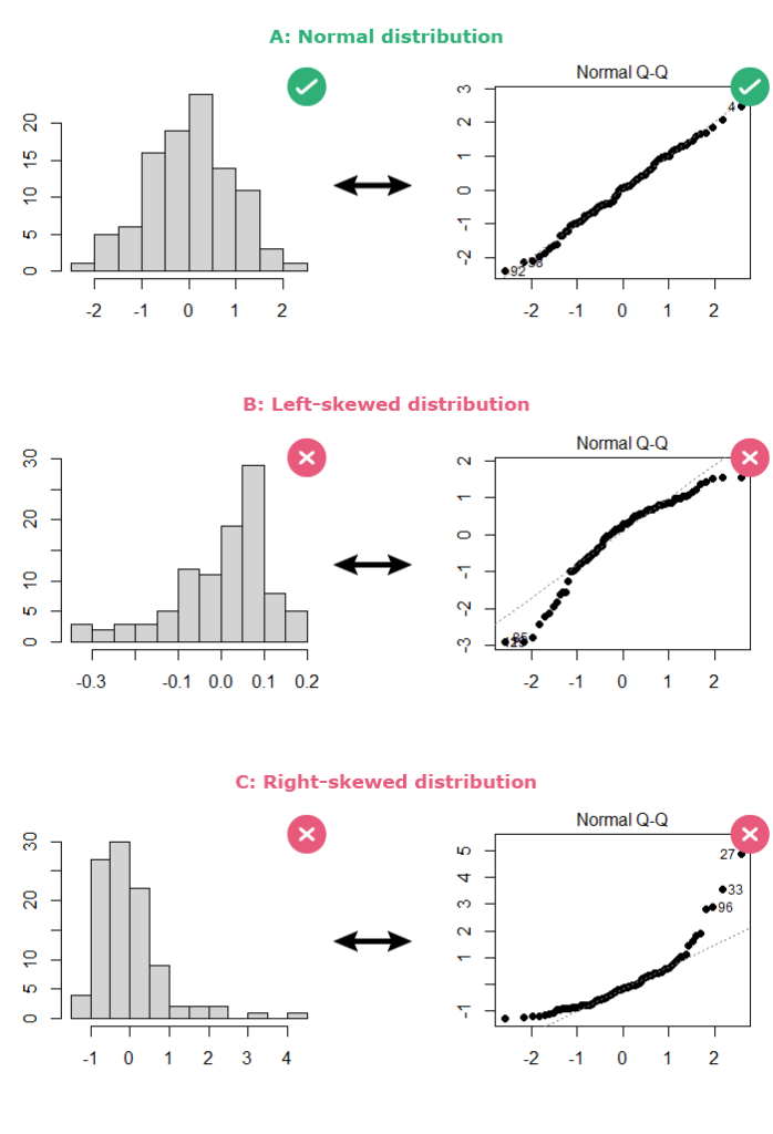
Look at Plot A (Normal distribution) in the image above. The points are not perfectly on the line, but they follow it very closely. This is what a "healthy" Q-Q plot looks like.
The "Bad" Plots: Deviations from Normality
When residuals are not normally distributed, the points will deviate from the reference line in a systematic way. Your job is to recognize these patterns. Here are the most common ones you'll encounter.

1. Skewness:
If the residuals are skewed, the points will form a curve or an arc.
- Positive (Right) Skew: The points curve up, falling above the reference line for high values and below the line for low values. See the "Positive skew" plot in the gallery above, and "Right-skewed distribution" (Plot C) in the first image. The highest and lowest residuals are further from the mean than a normal distribution would predict.
- Negative (Left) Skew: The points form an inverted curve. They fall below the reference line for high values and above the line for low values. See the "Negative skew" plot in the gallery and "Left-skewed distribution" (Plot B) in the first image.
2. Heavy or Light Tails (Kurtosis):
This refers to how many outliers your data has compared to a normal distribution. The pattern is often an "S" shape.
- Heavy Tails (Leptokurtic): Your data has more extreme outliers than a normal distribution would suggest. The Q-Q plot shows points pulling away from the reference line at both ends, forming a forward "S" shape. See the "Leptokurtic" plot in the gallery.
- Light Tails (Platykurtic): Your data has fewer outliers than expected. The Q-Q plot forms a horizontal "S" shape, with the tails bending inwards toward the center. See the "Platykurtic" plot in the gallery.
For your exam, distinguishing between positive and negative skew is the most critical skill. Recognizing heavy tails is also very useful.
This video provides an excellent visual summary of how to use the Q-Q plot and what these different deviations look like.
Simple Linear Regression: Diagnostics (part 4 of 4)
This video from the Biostatistics channel explains how to perform visual diagnostics for regression. We'll watch the segment focused specifically on the Q-Q plot.
Watch from this segment. The presenter first explains how to use the plot and then provides clear visual examples of what left skew, right skew, heavy-tailed, and light-tailed distributions look like on a Q-Q plot.
To solidify your understanding of these patterns, the following text provides detailed descriptions and illustrations.
This chapter gives a thorough breakdown of interpreting Q-Q plots. The simulations make the patterns very clear.
Start at section 8.6 Interpreting the Normal Q-Q Plot. Read the short intro, then focus on these key subsections: 8.6.2 Skew is indicated by monotonic curves...: This section shows clear examples of curved patterns for skewed data. 8.6.3 Direction of Skew: This explains how to tell left skew from right skew. 8.6.4 Outlier-proneness is indicated by “s-shaped” curves...: This covers the "S" shapes that indicate heavy and light tails.
Exam-Style Interpretation
Being able to write a concise and accurate conclusion is crucial.
-
If the plot looks good (normal):
The Normal Q-Q plot shows the points falling closely along the straight reference line. This supports the assumption that the residuals are normally distributed.
-
If the plot shows right skew:
The points on the Normal Q--Q plot form a U-shaped curve, indicating that the residuals are positively (right) skewed and violate the normality assumption.
-
If the plot shows heavy tails:
The points on the Normal Q-Q plot deviate from the reference line at both tails in an S-shape. This suggests the residuals are heavy-tailed (leptokurtic), violating the normality assumption.
A Note on Formal Tests: You might see a Shapiro-Wilk test for normality mentioned in some outputs. For your practical exam, relying on the visual evidence from the Q-Q plot is the standard and expected method. Formal tests can be overly sensitive to large sample sizes, flagging tiny, unimportant deviations. Stick to the plot.
Practice Drill
You are given the following Normal Q-Q plot from a regression analysis on student test scores.
Your Task:
- Assume the Q-Q plot for your model looks like the "Positive skew" plot in the image above. What does this plot tell you about the model's normality assumption? Write a one-sentence, exam-style conclusion.
Solution
Exam-Style Conclusion:
The Normal Q-Q plot shows a distinct curve where points are above the line at the top end and below the line at the bottom end, which indicates the residuals are positively skewed and violate the normality assumption.
Conclusion
You have now mastered the third of our four key diagnostic checks. You can now confidently assess linearity, homoscedasticity, and normality.
Key Takeaways:
- The Normal Q-Q plot is used to check if residuals are normally distributed.
- If the assumption is met, points will fall along the straight diagonal line.
- Curves indicate skewness (U-shape for positive skew, inverted U-shape for negative skew).
- "S" shapes indicate issues with the tails (heavy or light) compared to a normal distribution.
In our final lesson of this module, we will address the fourth assumption: the independence of residuals. This is especially important in data collected over time, where we must check for patterns like autocorrelation.