Understanding Interaction Effects in Regression Models

What is an Interaction Effect?

An interaction effect occurs when the relationship between a predictor variable and the outcome variable changes based on the level of a second predictor variable.

Think about food and condiments. The enjoyment you get from mustard depends heavily on the food you're putting it on.

• Mustard on a Hot Dog: Great! The effect of "mustard" on "enjoyment" is positive.
• Mustard on Ice Cream: Terrible. The effect of "mustard" on "enjoyment" is very negative.

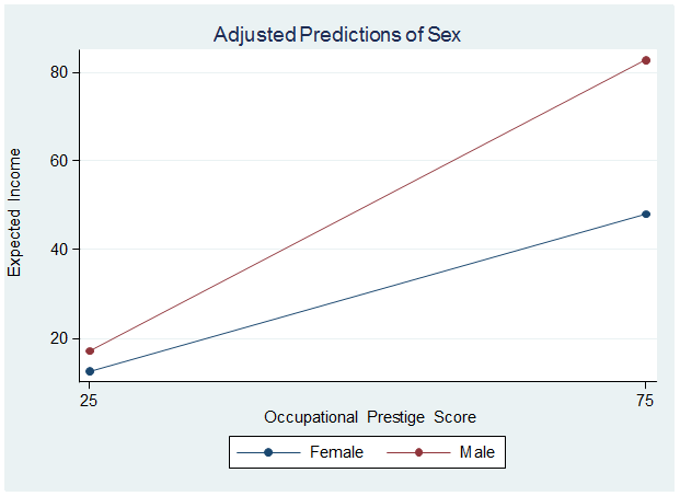
The effect of the condiment (mustard) depends on the food (hot dog vs. ice cream). This is an interaction. Visually, this is represented by non-parallel lines, as you can see in the plot below.

The Model with an Interaction Term

Let's consider a common case you'll see on your exam: the interaction between a continuous predictor (X) and a binary predictor (Z). The model equation is:

$\hat{Y}={\beta }_0+{\beta }_{1}X+{\beta }_{2}Z+{\beta }_3(X\cdot Z)$

Where:

• $X$ is our continuous variable (e.g., hours_studied).
• $Z$ is our dummy variable (e.g., is_private_school, coded 0 for Public, 1 for Private).
• $X\cdot Z$ is the interaction term.

The key to interpretation is to break this equation down for each category of the dummy variable.

Case 1: For the reference category (Z = 0, e.g., Public School)
If we plug in Z=0, the equation simplifies:
$\hat{Y}={\beta }_0+{\beta }_{1}X+{\beta }_2(0)+{\beta }_3(X\cdot 0)$
$\hat{Y}={\beta }_0+{\beta }_{1}X$
This is a simple linear equation.

• Intercept: ${\beta }_0$
• Slope: ${\beta }_1$

Case 2: For the other category (Z = 1, e.g., Private School)
If we plug in Z=1, we get:
$\hat{Y}={\beta }_0+{\beta }_{1}X+{\beta }_2(1)+{\beta }_3(X\cdot 1)$
Now, let's group the terms to see the new intercept and slope:
$\hat{Y}=({\beta }_0+{\beta }_2)+({\beta }_1+{\beta }_3)X$
This is also a linear equation, but with a different intercept and slope.

• Intercept: $({\beta }_0+{\beta }_2)$
• Slope: $({\beta }_1+{\beta }_3)$

How to Interpret the Coefficients (Exam Focus)

This is where you earn your marks. Let's define what each coefficient means in this context.

• ${\mathbf{\beta }}_0$ (Intercept): The predicted value of Y when both X=0 and Z=0 (i.e., for the reference group at the baseline level of the continuous predictor).
• ${\mathbf{\beta }}_1$ (Main Effect of X): The slope of X for the reference group only (when Z=0). It's the change in Y for a one-unit change in X, specifically for the group where Z=0.
• ${\mathbf{\beta }}_2$ (Main Effect of Z): The difference in the intercept between the group Z=1 and the reference group Z=0.
• ${\mathbf{\beta }}_3$ (Interaction Effect): This is the most important one. It is the difference in the slope of X for group Z=1 compared to group Z=0. It tells you how much the effect of X changes when you switch from the reference group to the other group.

Visually, an interaction means the lines representing the relationship for each group are not parallel.

Guided Walkthrough with R Output

Let's solidify this with a real example. The following video gives a great overview of the theory and how to specify the model in R. Pay close attention to how the presenter breaks down the model equation for each category.

Now, let's apply this to a detailed example from a public health dataset. We will use an excellent online textbook that walks through this step-by-step.

Let's dissect the R output from that reading together.

##                          Estimate Std. Error t value Pr(>|t|)
## (Intercept)                 2.209      0.503   4.396    0.000
## BMXWAIST                    0.040      0.005   8.276    0.000
## RIAGENDRFemale              1.746      0.649   2.690    0.007
## BMXWAIST:RIAGENDRFemale    -0.020      0.006  -3.218    0.001

Here, BMXWAIST is Waist Circumference (continuous) and RIAGENDRFemale is the dummy variable (0=Male, 1=Female).

Exam-Style Interpretation:

• BMXWAIST (${\beta }_1=0.040$): For males (the reference group), a 1 cm increase in waist circumference is associated with a 0.040 mmol/L increase in predicted fasting glucose.
• BMXWAIST:RIAGENDRFemale (${\beta }_3=-0.020$): The effect of waist circumference on predicted fasting glucose is 0.020 mmol/L lower for females than for males. The interaction is statistically significant (p = 0.001), so the relationship between waist circumference and fasting glucose significantly depends on gender.

Calculating the Slope for Females:

This directly addresses the second part of our learning outcome. To find the slope for females, we combine the main effect of BMXWAIST and the interaction effect:
${\text{Slope}}_{\text{Female}}={\beta }_1+{\beta }_3=0.040+(-0.020)=0.020$

So, for females, a 1 cm increase in waist circumference is associated with a 0.020 mmol/L increase in predicted fasting glucose.

Common Exam Trap: Misinterpreting Main Effects

As the reading and video emphasize, when an interaction term is in the model, the main effects cannot be interpreted as overall effects.

• The coefficient on BMXWAIST (0.040) is not the overall effect of waist circumference. It is only the effect for males.
• To state the effect of waist circumference, your answer must specify for which gender. The correct answer is, "The effect of waist circumference on fasting glucose depends on gender."

This next video brilliantly explains this trap and offers a simple way to think about it: to find the effect of a variable, just "gather up" all the terms in the equation that include that variable.

Practice Drill

You are given the following R output for a model predicting student exam_score based on hours_studied, program_type (0=STEM, 1=Arts), and their interaction.

Coefficients:
                             Estimate Std. Error t value Pr(>|t|)
(Intercept)                   55.20       2.10   26.29   <2e-16 ***
hours_studied                  4.50       0.50    9.00   <2e-16 ***
program_typeArts               7.30       3.00    2.43   0.016 *
hours_studied:program_typeArts -1.80       0.75   -2.40   0.017 *

Your Task:

1. What is the predicted effect of one additional hour of study on exam_score for a STEM student?
2. Write a one-sentence interpretation for the interaction term hours_studied:program_typeArts.
3. What is the predicted effect of one additional hour of study on exam_score for an Arts student?

Conclusion

You have just tackled one of the most complex but insightful aspects of linear regression. Mastering interactions separates a basic understanding from an advanced one and is a surefire way to impress on your exam.

Key Takeaways:

• An interaction means the effect of one predictor (X) on the outcome (Y) depends on the level of another predictor (Z).
• In a model $\hat{Y}={\beta }_0+{\beta }_{1}X+{\beta }_{2}Z+{\beta }_3(X\cdot Z)$, the main effect ${\beta }_1$ is the slope of X only for the reference group (Z=0).
• The interaction coefficient ${\beta }_3$ is the change in the slope of X when moving from the reference group to the other group (Z=1).
• To find the slope for the non-reference group, you must calculate ${\beta }_1+{\beta }_3$.

In our next lesson, we will cover the final topic in this module: log transformations. We will explore how they can help us model relationships that aren't linear and fix issues like heteroscedasticity, adding another powerful tool to our regression toolkit.